Diffraction peak detection
When the focused electron probe scans across a crystal, it creates a diffraction pattern at each scan position. In these patterns, we observe intense peaks (Bragg diffraction peaks) that act as fingerprints of the crystal structure. The positions of these diffraction peaks reveal information about atomic plane spacing and arrangement, while changes in their positions indicate crystal deformation. Accurate detection of these diffraction peaks is both crucial and challenging.
Understanding Bragg diffraction
Diffraction peaks appear in the pattern when electron waves scatter from sets of parallel atomic planes in the crystal. This process follows Bragg’s law:
- where:
d is the spacing between atomic planes
θ is the scattering angle
λ is the electron wavelength
n is an integer
Each diffraction peak in the pattern provides specific information:
Peak position: Reveals atomic plane spacing and orientation
Peak intensity: Indicates electron scattering strength
Peak displacement: Measures crystal deformation (strain)
Peak shape: Reflects crystal quality and thickness
Importance of accurate detection
The precision of our strain measurements depends directly on how accurately we can locate these diffraction peaks:
Strain sensitivity: A 0.1% strain shifts diffraction peaks by just 0.1% of their distance from the central beam
Signal-to-noise: True diffraction peaks must be distinguished from background noise
Pattern evolution: Diffraction peaks can appear, disappear, or change as the probe position changes
High throughput: A typical 4D-STEM dataset contains millions of diffraction peaks to analyze
Warning
Getting this wrong leads to:
False strain measurements
Missed deformations
Artifacts in strain maps
Incorrect structure determination
Locating diffraction peaks
Finding the exact centers of diffraction peaks accurately is both an art and a science. Over the years, researchers have developed increasingly sophisticated methods, each building on the insights and limitations of previous approaches. Let’s walk through this evolution, starting with the simplest but most robust method.
Challenges in diffraction peak detection
Several factors complicate accurate spot localization:
Intensity variations
Center spot much brighter than others
Weak spots barely above noise
Intensity changes with sample thickness
Spot shapes - Not perfectly circular - Can be distorted by aberrations - May overlap with neighbors
Background noise - Random detector noise - Diffuse scattering - Inelastic contributions
Pattern variations - Spots appear/disappear during scan - Intensity fluctuations - Sample drift effects
Center of mass: the foundation
The center of mass (COM) method was the first widely adopted approach, and it remains valuable for its simplicity and robustness. The concept is intuitive: treat each pixel’s intensity as a “weight” and find the weighted average position.
For a diffraction pattern \(I(x,y)\), the COM position is:
The method is particularly appealing because of its simplicity in Python:
# Method 1: Manual calculation
y_indices, x_indices = np.indices(pattern.shape)
total_intensity = np.sum(pattern)
x_com = np.sum(x_indices * pattern) / total_intensity
y_com = np.sum(y_indices * pattern) / total_intensity

# Method 2: Using scipy
from scipy.ndimage import center_of_mass
y_com, x_com = center_of_mass(pattern)
These limitations led to the development of more sophisticated detection methods, starting with Gaussian fitting.
Spot detection methods
Center of Mass (COM) - Fast but has limitations - Cannot distinguish pattern rotation from translation - Sensitive to intensity fluctuations - May jump discontinuously
Gaussian fitting Models diffraction spots with 2D Gaussian:
\[I(x,y) = A \exp\left(-\frac{(x-x_0)^2}{2\sigma_x^2} - \frac{(y-y_0)^2}{2\sigma_y^2}\right) + B\]where: - \((x_0,y_0)\): True center position - \(\sigma_x, \sigma_y\): Spot width - \(A\): Peak intensity - \(B\): Local background level
Drift and pattern evolution
Beyond detecting individual spots, a key challenge in 4D-STEM is monitoring how diffraction patterns change throughout the experiment. The center of mass (COM) method, despite its limitations for precise spot detection, proves valuable for tracking these global changes:
Sources of pattern evolution
Patterns can change during acquisition due to various factors:
Sample drift during scanning
Local crystal rotations
Strain fields
Thickness variations
Beam-induced damage
While COM tracking helps monitor these changes, it has specific limitations for drift analysis:
Cannot distinguish pattern rotation from translation
Sensitive to intensity fluctuations
May jump discontinuously if spots appear/disappear
The limitations of COM led to a key realization: we needed a method that could model the actual shape of diffraction spots. This brings us to the next evolution: Gaussian fitting.
Gaussian fitting: Modeling physical reality
As researchers delved deeper into electron diffraction, they realized that diffraction spots often follow a Gaussian-like intensity distribution. This isn’t just a mathematical convenience – it reflects the physical reality of how electrons scatter and how our detectors work.
The 2D Gaussian model attempts to capture the intensity distribution of diffraction spots:
where each parameter has physical significance: - \((x_0,y_0)\): The true center position we’re looking for - \(\sigma_x, \sigma_y\): Spot width, which relates to beam conditions - \(A\): Peak intensity, indicating scattering strength - \(B\): Local background level
Challenges in spot detection
While our mathematical framework for strain mapping is elegant, its practical implementation faces significant challenges. The success of strain measurement depends crucially on our ability to accurately locate diffraction spots in each pattern. However, real experimental data rarely matches the idealized case.
The Reality of Noise and Background
Real diffraction patterns emerge as complex superpositions of various signals—both desired and unwanted. Each scan position presents us with a pattern that contains not just the clean Bragg spots we seek, but also a multitude of other features that complicate our analysis:
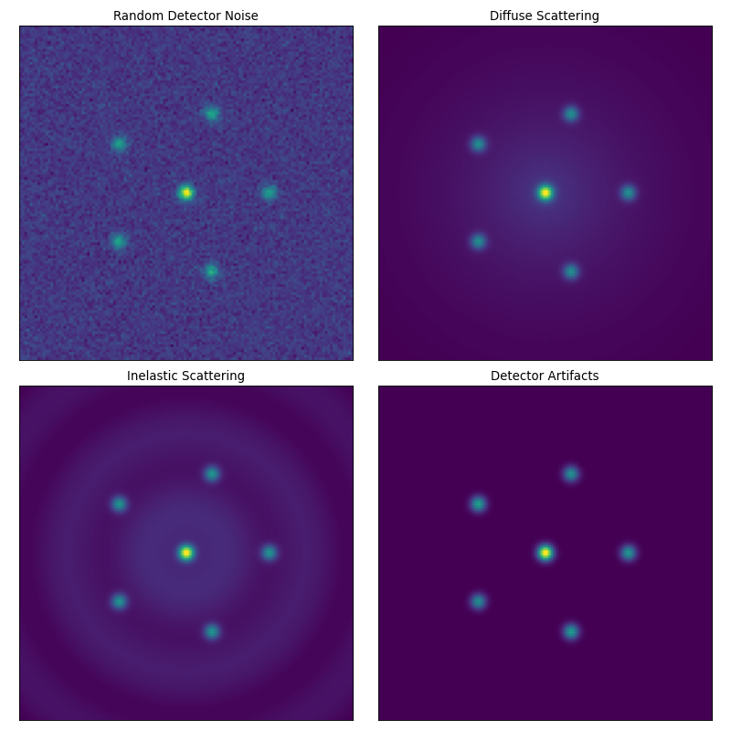
Different types of noise and artifacts in diffraction patterns. (a) Random detector noise showing Gaussian fluctuations. (b) Diffuse scattering background from thermal effects. (c) Inelastic scattering contributions. (d) Detector artifacts including dead pixels and gain variations.
Above each type of noise and artifact presents its own challenges. These effects are intrinsically linked to the physics of electron scattering (see quantum-electron-matter-interaction) and the practical limitations of our detectors:
Random detector noise (top left): Electronic noise in the detector creates a “salt-and-pepper” pattern of random intensity fluctuations. This noise follows a Gaussian distribution and can obscure weak diffraction spots.
Diffuse scattering background (top right): Thermal vibrations and disorder in the crystal create a smooth, radially-decreasing background intensity. This background can mask weak spots and complicate intensity measurements.
Inelastic contributions (bottom left): Electrons that lose energy through sample interactions create broad, diffuse features. These contributions are particularly strong in thicker samples or when imaging at lower voltages.
Detector artifacts (bottom right): Every detector brings its own set of imperfections to our measurements. Dead pixels create blind spots in our patterns, while variations in pixel sensitivity distort measured intensities. These systematic errors can create false peaks or subtly alter the apparent positions of real diffraction spots, directly impacting our strain calculations.
The challenge of intensity variations
A fundamental challenge in diffraction pattern analysis lies in the dramatic variations in spot intensities. This isn’t just a minor inconvenience—it’s a fundamental aspect of electron diffraction that stems from how electrons interact with the crystal.
This intensity variation creates several practical challenges:
Dynamic range: Modern detectors must handle intensity ratios of 1000:1 or greater between the central beam and weak diffraction spots.
Spot shape variations: Stronger spots often appear broader due to detector saturation or dynamic scattering effects, while weak spots may be sharp but barely above the noise level.
Overlapping features: When a strong spot lies near a weak one, the weak spot can be completely masked in the tail of the stronger spot.
The solution to these challenges often involves combining multiple approaches:
where \(I_{\text{scale}}\) is chosen to optimize the visibility of features across all intensity scales. This logarithmic transformation helps balance our competing needs: preserving the quantitative intensity information in strong spots while making weak spots visible for analysis.
Volume of Data: A typical 4D-STEM dataset might contain: - 256 × 256 scan positions - Each with a 512 × 512 diffraction pattern - Leading Well I’m not seeing the source code hereto millions of spots to analyze - Requiring automated processing
Over the years, researchers have developed increasingly sophisticated methods to address these challenges. Now let’s look at how these methods are applied in practice.
Drift and pattern evolution
Beyond detecting individual spots, a key challenge in 4D-STEM is monitoring how diffraction patterns change throughout the experiment. The center of mass (COM) method, despite its limitations for precise spot detection, proves valuable for tracking these global changes:
Sources of pattern evolution
Patterns can change during acquisition due to various factors:
Sample drift during scanning
Local crystal rotations
Strain fields
Thickness variations
Beam-induced damage
While COM tracking helps monitor these changes, it has specific limitations for drift analysis:
Cannot distinguish pattern rotation from translation
Sensitive to intensity fluctuations
May jump discontinuously if spots appear/disappear
These limitations in drift detection are distinct from the spot detection challenges discussed earlier, and they require their own specialized solutions.
The limitations of COM led to a key realization: we needed a method that could model the actual shape of diffraction spots. This brings us to the next evolution: Gaussian fitting.
Gaussian fitting: Modeling physical reality
As researchers delved deeper into electron diffraction, they realized that diffraction spots often follow a Gaussian-like intensity distribution. This isn’t just a mathematical convenience – it reflects the physical reality of how electrons scatter and how our detectors work.
The 2D Gaussian model attempts to capture the intensity distribution of diffraction spots:
where each parameter has physical significance: - \((x_0,y_0)\): The true center position we’re looking for - \(\sigma_x, \sigma_y\): Spot width, which relates to beam conditions - \(A\): Peak intensity, indicating scattering strength - \(B\): Local background level
Handling Multiple Spots
In real diffraction patterns, we need to analyze many spots simultaneously. The process typically involves:
Spot detection: Find potential spot locations using local maxima
Patch extraction: Cut out small regions around each spot
Individual fitting: Fit a Gaussian to each patch independently
Quality control: Validate fits using R² scores and other metrics
Key advantages of patch-based fitting:
Sub-pixel accuracy: By fitting a continuous function, we can locate centers with precision better than our pixel size
Noise resilience: The fit naturally averages out random noise, giving more reliable positions
Shape information: The \(\sigma\) parameters tell us about spot quality and beam conditions
However, Gaussian fitting also introduced new challenges:
Computational cost: Fitting is an iterative process, much slower than COM - Each spot needs ~10-100 iterations to converge - Each iteration involves evaluating exponentials - A single pattern might have dozens of spots
Initial guess required: The fit needs a starting point - Often use COM for initial position - Bad guesses can lead to failed convergence - Multiple spots can confuse the optimizer
These limitations led to an important insight: we needed a method that could handle more complex spot shapes while maintaining computational efficiency. This realization led to the development of template matching approaches.
Template matching: The power of pattern recognition
The next breakthrough in spot detection came from a seemingly simple observation: humans are remarkably good at recognizing diffraction spots because we know what they should look like. This insight led to template matching, where we use a known “template” of a diffraction spot to find similar patterns in the data.
The core of template matching is cross-correlation—a mathematical way to measure how well a template matches different parts of an image. For a template \(T(x,y)\) and a diffraction pattern \(I(x,y)\), the cross-correlation is:
High values of \(C(x,y)\) indicate likely spot locations. The beauty of this approach lies in its flexibility with templates. Researchers can use:
This adaptability made template matching particularly powerful for complex situations where simple Gaussian models fall short. For instance, when dealing with asymmetric spots from sample tilt, the template can capture this asymmetry. When spots have characteristic internal structure from dynamical diffraction, the template preserves this information.
However, template matching brought its own set of challenges. The quality of your results depends critically on how well your template matches reality. A mismatched template can miss important spots or generate false positives. Furthermore, the computational cost is significant—you’re essentially sliding the template across every possible position in your diffraction pattern.
Hybrid methods: Combining the best of all worlds
As our understanding of spot detection evolved, researchers realized that no single method was perfect for all situations. This led to the development of hybrid approaches that combine multiple techniques in a strategic sequence. The key insight was that different methods excel at different aspects of the problem.
A typical hybrid workflow exploits this complementarity:
Start with template matching to find candidate spots, leveraging its ability to identify spots even in noisy or complex patterns
Use center of mass for a quick, rough position estimate—it’s fast and provides a good starting point
Finish with Gaussian fitting for high precision, now that we have a good initial guess
This sequence is analogous to how a human expert might work: first spotting patterns visually (like template matching), then roughly centering their attention (like COM), and finally carefully determining the exact center (like Gaussian fitting).
Advanced processing and tracking
As we scan across the sample, we must track how diffraction spots move and change. This is similar to tracking stars across astronomical plates, but with an important difference—our “stars” (diffraction spots) can appear, disappear, or change intensity as the crystal orientation and strain state varies.
We record each spot’s position as a reciprocal space vector:
The challenge lies in maintaining consistency—ensuring we’re tracking the same family of spots across the entire scan. This requires sophisticated bookkeeping algorithms that can:
Match spots between adjacent scan positions
Handle spots that temporarily disappear
Account for large changes near crystal defects
The quality of this tracking directly impacts our final strain resolution.
The reference pattern challenge
One of the most critical challenges in strain mapping is establishing a reliable reference state. This challenge stems from a fundamental question: what do we consider “unstrained”? In theory, we need a perfect crystal structure with zero deformation, but in practice, this ideal scenario rarely exists. Let’s explore the various approaches to this challenge, their limitations, and practical solutions.
The experimental reference approach
The most straightforward approach is to find an “unstrained” region in your sample. But this raises several practical questions:
How do we identify truly unstrained regions?
What if the entire sample is strained?
How do we account for sample-to-sample variations?
In practice, researchers typically choose reference regions based on these strategies:
Edge regions: Areas far from obvious strain sources (interfaces, defects) are often used as references. The assumption is that strain fields decay with distance, so remote regions should be relatively unstrained. However, this assumption can break down if: - The sample has residual strain from processing - Edge effects influence the local structure - Long-range strain fields exist
Known structures: If your sample contains a well-characterized region (like a substrate with known lattice parameters), this can serve as a reference. But beware: - Even “perfect” substrates may have surface relaxation - Thin film samples might have substrate bending - Temperature differences can cause thermal strain
Control samples: Sometimes, preparing a separate unstrained reference sample is necessary. This works well when: - You can make identical ../materials under controlled conditions - The processing doesn’t introduce strain - The reference sample is stable during measurement
Pattern averaging: Dealing with noise
Once you’ve identified a reference region, the next challenge is getting reliable diffraction data. Single diffraction patterns are often too noisy for precise measurements. The solution is pattern averaging, but this isn’t as simple as it sounds:
First, you need to confirm pattern consistency: - Check that spot positions don’t drift - Verify intensity distributions are stable - Look for any systematic variations
Then, implement smart averaging: - Align patterns to account for small shifts - Weight patterns based on quality metrics - Remove outliers that could skew results
Finally, validate the averaged pattern: - Compare with theoretical predictions - Check symmetry relationships - Estimate uncertainty in spot positions
Like an aging camera, detectors develop their own quirks and imperfections over time. Understanding these quirks is crucial for separating the true signal from the detector’s personal signature.
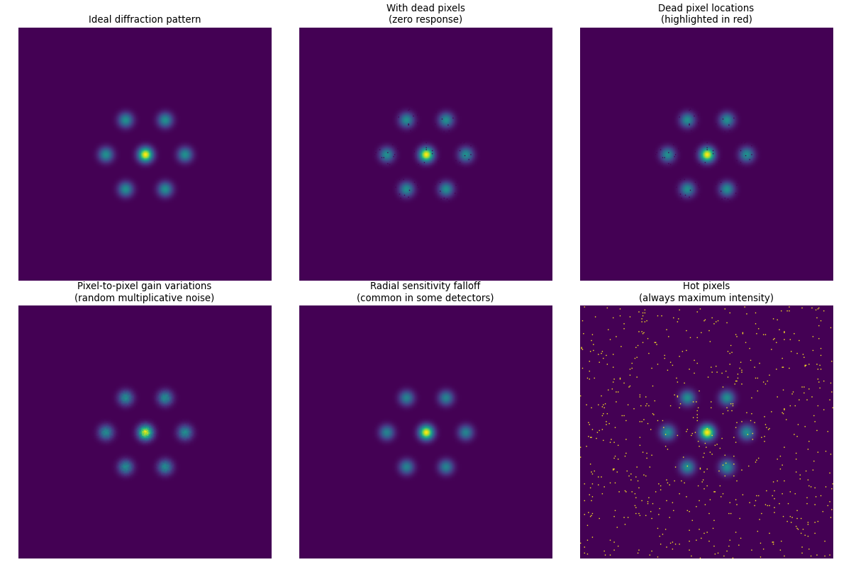
How detectors see the world. Left: The perfect vision we want. Right: The reality we get, complete with blind spots (dead pixels), uneven sensitivity (gain variations), and hot spots.