CUDA fundamentals
This page covers CUDA C++ programming fundamentals for GPU computing. Content is based on the NVIDIA CUDA C++ Programming Guide and tutoring sessions with LLMs.
Note
Looking for hands-on tutorials? See CUDA tutorials for 7 progressive examples from basic 2D matrix operations to production-ready pipelined processing with CUDA streams.
Learning roadmap
Core fundamentals shared in this page.
[x] CPU–GPU memory architecture and data transfers
[ ] 2D matrix operations with CUDA
[ ] Parallelizing computation across threads
[ ] Configuring blocks and grids for large data
[ ] Optimizing memory access patterns
[ ] Using shared memory for performance gains
[ ] Synchronization and avoiding race conditions
[ ] Profiling and debugging CUDA kernels
[ ] Streams and overlapping computation with data transfer
[ ] Tiling techniques for matrix multiplication
[ ] Warp-level programming and intrinsics
[ ] Mixed precision and tensor cores
[ ] CUDA libraries (cuBLAS, cuDNN, Thrust)
Here are some topics beyond covered above. As I learn more, I will document them throuhgout my website.
The full disciplinary stack (from bottom to top)
Understanding where CUDA fits in the complete computing stack:
Quantum and solid-state physics (electron behavior)
Semiconductor materials science (how transistors are built)
Device and VLSI engineering (how circuits are designed)
Computer architecture (how logic becomes compute units)
System architecture (how chips form clusters)
Compiler and runtime systems (how code maps to hardware)
Parallel programming models (CUDA, etc. — how you control it)
Numerical methods and algorithms (what problems you solve)
Scientific application domains (where GPU computing changes the world)
Intermediate level
Occupancy and scheduling
Occupancy modeling (how register pressure and shared memory affect SM concurrency)
Memory hierarchy deep dive (L1/L2 caching, prefetching, memory coalescing with hardware cache lines)
Asynchronous memory transfers and CUDA Graphs API (building dependency graphs for complex workflows)
Numerical and algorithmic optimization
Sparse linear algebra on GPUs (CSR, COO, ELL formats, SpMV kernels)
FFT and spectral methods (cuFFT and custom transforms)
Stencil computations and PDE solvers (time-stepping, ghost cells, halo exchange)
Monte Carlo methods (parallel RNGs like Philox, XORWOW, Sobol)
Reduction and scan patterns (warp-shuffle vs shared memory, hierarchical reductions)
Multi-GPU and distributed computing
NVLink and PCIe topology tuning
Unified Virtual Addressing (UVA) and peer-to-peer access
Multi-GPU programming with NCCL and MPI (domain decomposition, collective communication)
GPU clusters and CUDA-aware MPI (scaling scientific solvers to supercomputers)
Performance engineering and tools
Roofline analysis (quantifying compute vs bandwidth bounds)
CUDA Nsight Compute and Nsight Systems (instruction throughput, stalls, dependency graphs)
PTX/SASS inspection (reading compiler output to tune instruction-level behavior)
Autotuning frameworks (search-based kernel optimization like OpenTuner, Kernel Tuner)
Advanced language and ecosystem topics
CUDA with OpenMP/OpenACC interoperability
HIP and SYCL portability (writing kernels that run on AMD/Intel GPUs)
CUDA Graphs and Cooperative Groups
Dynamic parallelism (kernels launching kernels)
C++20 features in CUDA (templates, constexpr, thrust-style metaprogramming)
Python GPU bindings (Numba, CuPy, PyTorch extensions, CFFI bridges)
Domain-specific scientific applications
Finite element and finite volume GPU implementations
Molecular dynamics (LAMMPS, GROMACS implementations)
GPU-accelerated signal and image processing
Machine learning kernels (matrix multiply to custom activation and gradient ops)
Hybrid CPU–GPU solvers (splitting work between CPU control and GPU compute)
Research-level and experimental directions
Persistent kernels and task-based execution models
Graph and irregular computation on GPUs
GPU–CPU co-scheduling for heterogeneous architectures
Memory compression and precision-adaptive computing
Quantum-inspired and tensor network algorithms on GPU
Advanced level
GPU compiler and low-level architecture mastery
PTX-to-SASS compilation pipelines (learn how nvcc, ptxas, and driver JIT interact)
LLVM and NVVM IR (understanding CUDA’s compiler backend for custom IR passes)
Binary instrumentation tools (NVBit, CUPTI for runtime analysis at instruction granularity)
Register allocation and instruction scheduling (hardware scoreboards, dependencies, latency hiding)
Dynamic kernel specialization (JIT compiling PTX at runtime for adaptive workloads)
Advanced parallel algorithm design
GPU graph analytics (frontier-based BFS, PageRank, sparse gather-scatter, libraries like Gunrock)
Irregular memory access optimization (handling unstructured meshes and adaptive grids efficiently)
Load balancing and work redistribution (dynamic task assignment across warps or GPUs)
Parallel prefix sums, scans, and reductions for high-dimensional data
Asynchronous collective operations (overlapping computation with communication in multi-GPU systems)
System-level and HPC integration
GPUDirect RDMA (direct GPU-to-NIC communication for low-latency distributed HPC)
GPUDirect Storage (bypassing CPU for I/O-intensive workflows like HDF5, netCDF, large dataset streaming)
CUDA in containerized and cloud environments (Singularity, Docker with NVIDIA runtime, Kubernetes scheduling)
Slurm and job scheduler integration for GPU clusters
NUMA and CPU pinning for heterogeneous performance optimization
Advanced numerical computing and scientific software design
Mixed-precision iterative refinement (combining FP16/FP32/FP64 arithmetic intelligently)
GPU-accelerated preconditioners (AMG, ILU, domain-decomposition methods)
Automatic differentiation at kernel level (custom gradient operators for scientific ML or differentiable simulators)
Spectral element and discontinuous Galerkin methods (GPU mapping of high-order basis functions)
Adaptive mesh refinement (AMR) frameworks with dynamic data redistribution between GPUs
Cross-domain acceleration and frontier hardware
CUDA with TensorRT and cuQuantum (domain fusion for ML and physics simulations)
Hopper and Blackwell architecture deep dives (tensor memory accelerator, FP8 formats, DPX instructions)
FPGA–GPU hybrid workflows (offloading pre/post-processing to FPGAs or DPU units)
Heterogeneous memory systems (HBM3 vs GDDR7 tradeoffs, Unified Memory oversubscription tuning)
Meta-programming and performance portability
Template metaprogramming for kernel generation (compile-time specialization for problem dimensions)
Code generation frameworks (building your own mini-Thrust or Tensor compiler)
Performance portability layers (Kokkos, RAJA, and their CUDA backends)
AutoML for kernel optimization (AI-guided parameter tuning and kernel fusion)
Research and exascale computing
Exascale GPU programming models (evolving standards like OpenMP 5, SYCL 2.0, CUDA Graphs 2.0)
Fault tolerance on GPUs (checkpointing, redundant computation, resilience to transient faults)
Energy-efficient GPU computing (DVFS tuning, instruction-level power modeling)
Domain decomposition at exascale (overlapping communication, topology-aware scheduling)
Expert level
GPU compiler and low-level architecture mastery
PTX-to-SASS compilation pipelines (learn how nvcc, ptxas, and driver JIT interact)
LLVM and NVVM IR (understanding CUDA’s compiler backend for custom IR passes)
Binary instrumentation tools (NVBit, CUPTI for runtime analysis at instruction granularity)
Register allocation and instruction scheduling (hardware scoreboards manage dependencies and latency hiding)
Dynamic kernel specialization (JIT compiling PTX at runtime for adaptive workloads)
Advanced parallel algorithm design
GPU graph analytics (frontier-based BFS, PageRank, sparse gather-scatter, libraries like Gunrock)
Irregular memory access optimization (handling unstructured meshes and adaptive grids efficiently)
Load balancing and work redistribution (dynamic task assignment across warps or GPUs)
Parallel prefix sums, scans, and reductions for high-dimensional data
Asynchronous collective operations (overlapping computation with communication in multi-GPU systems)
System-level and HPC integration
GPUDirect RDMA (direct GPU-to-NIC communication for low-latency distributed HPC)
GPUDirect Storage (bypassing CPU for I/O-intensive workflows like HDF5, netCDF, large dataset streaming)
CUDA in containerized and cloud environments (Singularity, Docker with NVIDIA runtime, Kubernetes scheduling)
Slurm and job scheduler integration for GPU clusters
NUMA and CPU pinning for heterogeneous performance optimization
Advanced numerical computing and scientific software design
Mixed-precision iterative refinement (combining FP16/FP32/FP64 arithmetic intelligently for speed and accuracy)
GPU-accelerated preconditioners (AMG for algebraic multigrid, ILU, domain-decomposition methods)
Automatic differentiation at kernel level (custom gradient operators for scientific ML or differentiable simulators)
Spectral element and discontinuous Galerkin methods (GPU mapping of high-order basis functions)
Adaptive mesh refinement (AMR) frameworks with dynamic data redistribution between GPUs
Cross-domain acceleration and frontier hardware
CUDA with TensorRT and cuQuantum (domain fusion for ML and physics simulations)
Hopper and Blackwell architecture deep dives (tensor memory accelerator, FP8 formats, DPX instructions)
FPGA–GPU hybrid workflows (offloading pre/post-processing to FPGAs or DPU units)
Heterogeneous memory systems (HBM3 vs GDDR7 tradeoffs, Unified Memory oversubscription tuning)
Meta-programming and performance portability
Template metaprogramming for kernel generation (compile-time specialization for problem dimensions)
Code generation frameworks (building your own mini-Thrust or Tensor compiler)
Performance portability layers (Kokkos, RAJA, and their CUDA backends)
AutoML for kernel optimization (AI-guided parameter tuning and kernel fusion)
Research and exascale computing
Exascale GPU programming models (evolving standards like OpenMP 5, SYCL 2020, CUDA Graphs 2.0)
Fault tolerance on GPUs (checkpointing, redundant computation, resilience to transient faults)
Energy-efficient GPU computing (DVFS tuning, instruction-level power modeling)
Domain decomposition at exascale (overlapping communication, topology-aware scheduling)
Beyond CUDA
Hardware-software co-design
SM microarchitecture design (studying warp schedulers, register file banking, SIMT divergence handling at RTL or simulator level)
Cache-coherence protocol simulation (using GPGPU-Sim, Multi2Sim, or Accel-Sim to test new GPU memory hierarchies)
Custom GPU ISA extensions (experimenting with new PTX opcodes, tensor instructions, or synchronization primitives)
Energy–performance tradeoff modeling (designing kernels that exploit power gating and clock domain scaling)
Compiler and runtime research
Custom CUDA frontends (using Clang/LLVM to emit NVVM or PTX directly)
MLIR and Polyhedral optimization (building domain-specific GPU compilers for PDEs, quantum simulation, or graph analytics)
Kernel fusion and scheduling research (compiler passes that reorder kernels for maximum cache reuse and minimal global memory trips)
Auto-schedulers and learned compiler models (like TVM or Triton, where AI models learn to generate optimized kernels)
Custom runtime systems (adaptive task graphs, persistent kernel scheduling frameworks beyond CUDA Graphs)
Next-generation parallel models
Task-based and dataflow execution models (Legion, PaRSEC, Charm++, Kokkos with HPX)
Asynchronous many-task (AMT) runtime research (overlapping thousands of fine-grained GPU tasks)
Heterogeneous memory systems (disaggregated memory and CXL Compute Express Link for GPU clusters)
Speculative parallelism and transactional memory on GPUs
Numerical methods and exascale algorithms
Mixed-precision stability theory (rigorous analysis of error propagation in hybrid-precision solvers)
Resilient iterative methods (algorithms that recover from bit flips or soft errors during GPU execution)
Asynchronous numerical methods (time-stepping without global synchronization barriers)
GPU-accelerated quantum simulation (tensor network contraction, variational algorithms, quantum circuit simulation at scale)
Adaptive multiphysics frameworks (dynamic load balancing between solvers like fluid, chemistry, radiation on GPUs)
Cross-disciplinary HPC research
AI and HPC fusion (neural operators, differentiable physics, scientific machine learning SciML)
Physics-informed neural networks (PINNs with custom GPU kernels for PDE learning)
Quantum–classical hybrid systems (CUDA interacting with QPUs or FPGA accelerators)
Data-driven compiler optimization (reinforcement learning tuning compiler flags and kernel schedules)
Exascale visualization pipelines (GPU-based volume rendering of petabyte-scale simulation data)
Emerging paradigms
Analog and optical accelerators (using GPU-like APIs to control optical tensor cores or analog compute arrays)
Neuromorphic co-processing (integrating CUDA with spiking neural hardware for asynchronous event-driven simulation)
GPU simulators for future ISAs (building the next CUDA for post-von-Neumann systems)
Software-defined GPUs (virtual GPU orchestration across datacenters, abstracting away physical hardware)
Heterogeneous exascale orchestration (co-scheduling GPUs, TPUs, and quantum nodes via unified runtime models)
Fundamental concepts
- What is CUDA?
CUDA (Compute Unified Device Architecture) is NVIDIA’s parallel computing platform and programming model that enables developers to use GPUs for general-purpose computing. It extends C++ with keywords to define GPU functions (kernels) and manage device memory.
- What is a kernel?
A kernel is a function that runs on the GPU, defined using the
__global__qualifier. It can be called from CPU code and executes in parallel across many GPU threads.- What is heterogeneous programming?
Heterogeneous programming refers to using different types of processors (CPUs and GPUs) within a single application to leverage their unique strengths. In CUDA, this means writing code that runs on both the host (CPU) and device (GPU), allowing parallel processing and acceleration of compute-intensive tasks.
- How are CUDA threads organized?
CUDA threads are organized hierarchically:
Thread: The smallest unit of execution
Block: A group of threads that can cooperate via shared memory
Grid: A collection of blocks launched by a single kernel
Cluster: (compute capability 9.0+) A group of blocks that share memory
Threads are specified using
<<<numBlocks, threadsPerBlock>>>syntax.- What is
threadIdx? Built-in variable containing the thread index within its block. For multi-dimensional blocks, access components as
threadIdx.x,threadIdx.y,threadIdx.z.- What is
blockIdx? Built-in variable containing the block index within the grid. For multi-dimensional grids, access components as
blockIdx.x,blockIdx.y,blockIdx.z.- What is
blockDim? Built-in variable containing the dimensions (number of threads) of a block in each dimension (x, y, z).
- How is memory shared at different thread hierarchy levels?
Memory sharing follows the thread hierarchy. Each thread has private registers, threads within a block share block-level shared memory, and all threads can access grid-level global memory. This hierarchy exists because registers are fastest (1 cycle) but limited in size, while global memory is slow (hundreds of cycles) but large. See the Memory hierarchy section below for detailed performance characteristics and visualization.
Memory hierarchy and performance
- What is memory coalescing?
Memory coalescing occurs when consecutive threads access consecutive memory addresses, allowing the GPU to fetch all data in a single memory transaction. This dramatically improves performance.
Memory transaction visualization:
GPU Memory Bus (32-byte transactions): Address: 1000 1004 1008 1012 1016 1020 1024 1028 ┌─────┬─────┬─────┬─────┬─────┬─────┬─────┬─────┐ Memory: │ A0 │ A1 │ A2 │ A3 │ A4 │ A5 │ A6 │ A7 │ └─────┴─────┴─────┴─────┴─────┴─────┴─────┴─────┘ └──────────────── One transaction ───────────────┘ (32 bytes = 8 floats) Coalesced access (GOOD): Thread 0 → A0 (1000) Thread 1 → A1 (1004) Thread 2 → A2 (1008) Thread 3 → A3 (1012) Result: ONE memory transaction for all 4 threads Scattered access (BAD): Thread 0 → A0 (1000) ─┐ Thread 1 → A4 (1016) ├─ Three separate transactions Thread 2 → A8 (1032) ─┘ Result: THREE memory transactions for 3 threads- Why does row-major layout enable coalescing?
When processing a 2D array row by row, consecutive threads naturally access consecutive memory locations, enabling coalesced access.
Column-major vs row-major access:
2D array in memory (row-major):
0   1   2   3   4   5   6   7   8   9  10  11
└───Row 0───┘└───Row 1───┘└───Row 2───┘

Accessing by rows (coalesced):
Thread 0 → index 0 ┐
Thread 1 → index 1 ├─ Consecutive addresses
Thread 2 → index 2 ┘   ONE transaction

Accessing by columns (scattered):
Thread 0 → index 0 (row 0) ┐
Thread 1 → index 4 (row 1) ├─ Large gaps between addresses
Thread 2 → index 8 (row 2) ┘   Multiple transactions
- What is shared memory in CUDA?
Shared memory is fast, on-chip memory that can be accessed by all threads within a block. It enables threads to cooperate by sharing intermediate results, reducing expensive global memory accesses.
- What is
__syncthreads()? A barrier synchronization function that ensures all threads in a block reach the same point before proceeding. Essential when using shared memory to prevent race conditions.
Thread hierarchy
- What are thread block clusters?
Thread block clusters (compute capability 9.0+) are groups of thread blocks that can share data within a kernel. Clusters provide an intermediate level of organization between blocks and the full grid.
Thread hierarchy levels:
Grid (entire kernel launch)
├── Cluster (group of blocks)
│   ├── Block (group of threads)
│   │   ├── Thread 0
│   │   ├── Thread 1
│   │   └── ...
│   └── Block
│       └── Threads...
└── Cluster
    └── Blocks...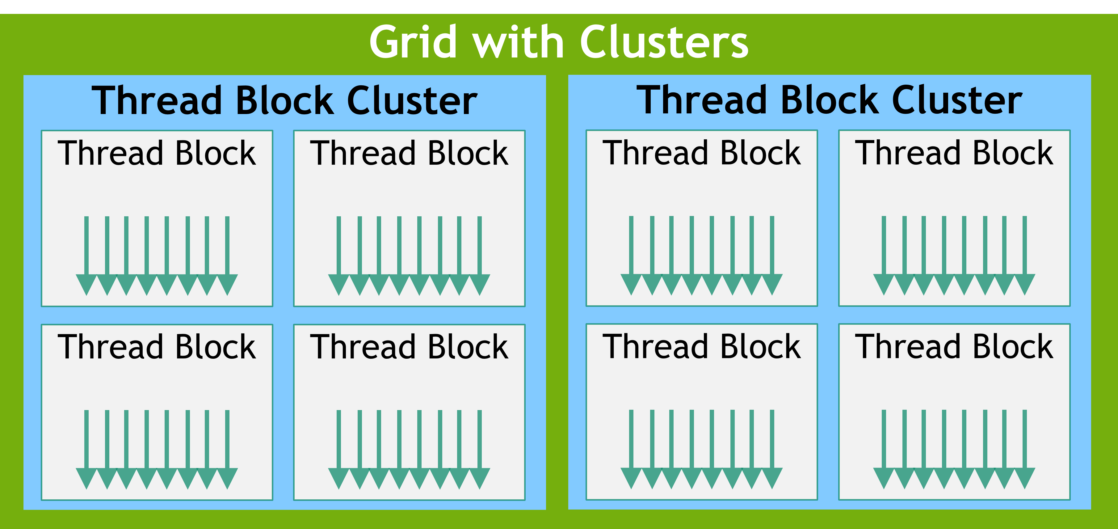
Grid of thread block clusters (source: NVIDIA)
- How do you specify cluster dimensions?
Use the
__cluster_dims__(x, y, z)qualifier in the kernel definition to specify compile-time cluster size.// Cluster with 2 blocks in X dimension, 1 in Y and Z __global__ void __cluster_dims__(2, 1, 1) cluster_kernel(float *input, float* output) { // Kernel code } int main() { dim3 threadsPerBlock(16, 16); dim3 numBlocks(N / 16, N / 16); // Grid dimension must be multiple of cluster size cluster_kernel<<<numBlocks, threadsPerBlock>>>(input, output); }
- What is the maximum cluster size?
Cluster size limits are hardware dependent. For NVIDIA A100 GPUs, the maximum is 8 blocks in each dimension (X, Y, Z). Check your specific GPU architecture documentation for limits.
Memory hierarchy
- What are the memory types in CUDA?
CUDA provides several memory types with different scopes, lifetimes, and performance characteristics.
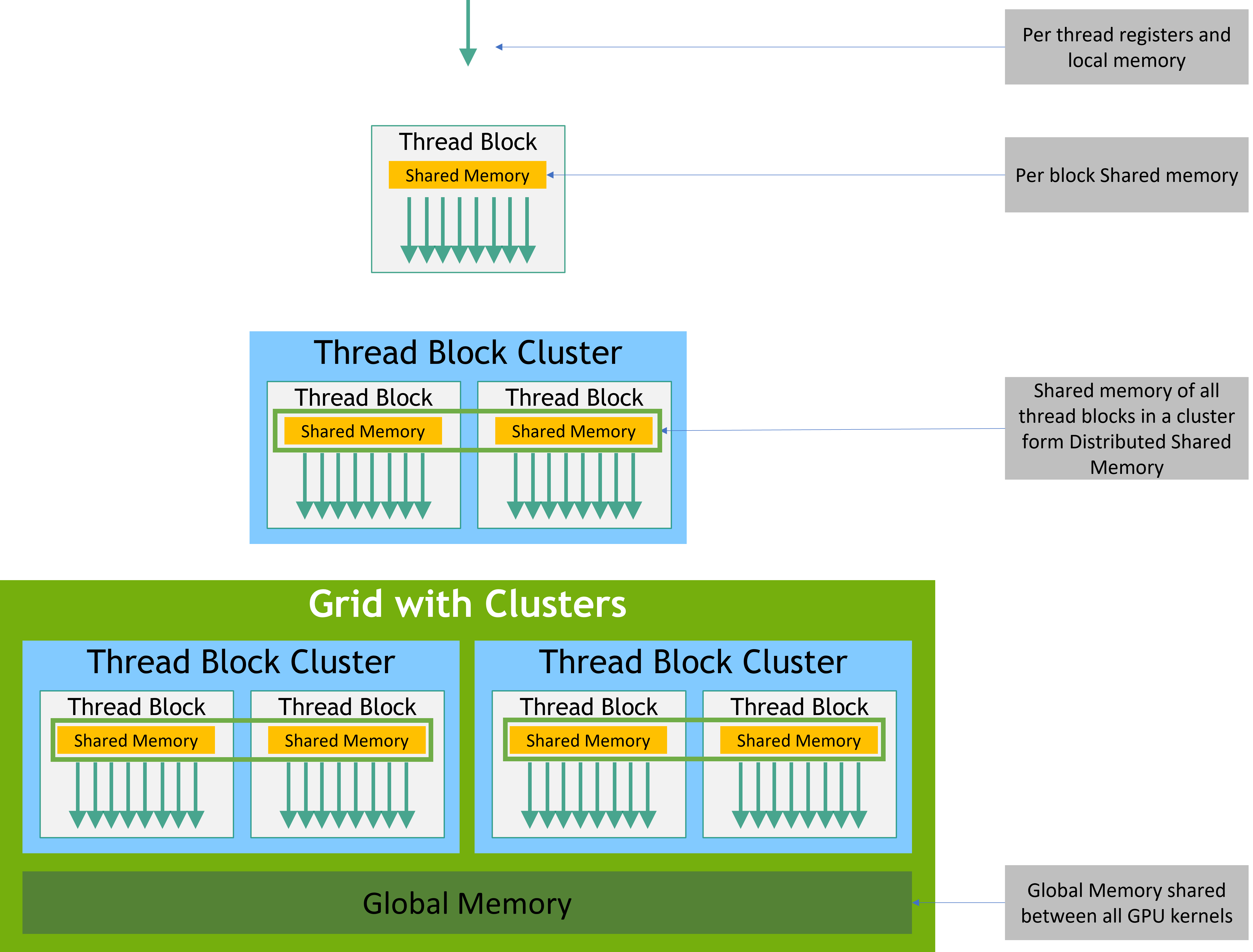
CUDA memory hierarchy (source: NVIDIA)
Memory hierarchy table:
Memory Type
Scope
Lifetime
Speed
Use Case
Registers
Thread
Thread
Fastest
Local variables
Shared Memory
Block
Block
Very Fast
Thread cooperation
Global Memory
Grid
Application
Slow
Large datasets
Constant Memory
Grid
Application
Fast (cached)
Read-only data
Texture Memory
Grid
Application
Fast (cached)
Spatial locality
Memory sharing visualization:
Grid
┌────────────────────────────────────────────────┐
│  Global Memory (all blocks can access)         │
│  ┌──────────────┐     ┌──────────────┐         │
│  │ Block 0      │     │ Block 1      │         │
│  │ Shared Mem 0 │     │ Shared Mem 1 │         │
│  │ ┌──┐  ┌──┐   │     │ ┌──┐  ┌──┐   │         │
│  │ │T0│  │T1│   │     │ │T0│  │T1│   │         │
│  │ │R │  │R │   │     │ │R │  │R │   │         │
│  │ └──┘  └──┘   │     │ └──┘  └──┘   │         │
│  └──────────────┘     └──────────────┘         │
└────────────────────────────────────────────────┘

R = Thread private registers (fastest, private to each thread)
T0, T1 = Different threads within a block
Shared Mem = Accessible by all threads in block (very fast)
Global Memory = Accessible by all threads in grid (slow)
- Why does this memory hierarchy exist?
Performance: Registers are fastest (1 cycle), shared memory is very fast (few cycles), global memory is slow (hundreds of cycles)
Hardware constraints: GPU streaming multiprocessors (SMs) have limited on-chip memory, so shared memory must be divided among active blocks
Programming model: Block-level sharing enables efficient cooperation algorithms (reductions, prefix sums) while grid-level sharing allows communication across the entire problem
Compilation
- What is nvcc?
The NVIDIA CUDA Compiler (nvcc) compiles CUDA C/C++ code into executable binaries that run on NVIDIA GPUs. It handles both host (CPU) code and device (GPU) code, generating optimized machine code for each.
- What is just-in-time (JIT) compilation?
JIT compilation compiles code at runtime rather than ahead of time. In CUDA, this enables dynamic optimization and GPU code generation based on specific hardware and runtime conditions.
- When is JIT compilation useful in machine learning?
JIT compilation is valuable when deploying models across different GPU architectures. PyTorch’s
torch.jit.scriptandtorch.jit.tracecompile models at runtime, optimizing operations (matrix multiplications, convolutions, custom kernels) for the target GPU’s compute capability. Examples include SM_80 for A100 and SM_86 for RTX 3090. This allows the same model code to run efficiently on different hardware without manual recompilation.
Memory management
- What is linear memory?
Linear memory is a contiguous block of memory allocated on the GPU. It is the most common memory type for storing data arrays in CUDA programs and can be accessed efficiently by threads using simple indexing.
- How do you allocate and free GPU memory?
Use
cudaMalloc()to allocate memory on the device andcudaFree()to release it.float* d_A; size_t size = N * sizeof(float); // Allocate memory on GPU cudaMalloc(&d_A, size); // Use memory... // Free memory cudaFree(d_A);
- How do you copy data between host and device?
Use
cudaMemcpy()to transfer data between CPU (host) and GPU (device) memory.// Copy direction flags: cudaMemcpyHostToDevice // CPU → GPU cudaMemcpyDeviceToHost // GPU → CPU cudaMemcpyDeviceToDevice // GPU → GPU
Memory
What is the concept of “Linear memory” in CUDA?
Linear memory refers to a contiguous block of memory allocated on the GPU that can be accessed by threads in a straightforward manner. It is the most common type of memory used for storing data arrays in CUDA programs.
What API is used to allocate and free linear memory in CUDA?
cudaMalloc() to allocate linear memory on the GPU and cudaFree() to free that memory.
How do you copy data between host and device memory in CUDA?
Usethe cudaMemcpy() function to copy data between host (CPU) memory and device (GPU) memory.
- What is the complete workflow for a CUDA program?
A typical CUDA program follows this pattern: allocate host memory, allocate device memory, copy data to device, launch kernel, copy results back, and free memory.
Memory workflow visualization:
Step 1: Allocate host memory (CPU)
┌─────────────────────────────────────┐
│ CPU Memory (Host)                   │
│ ┌──────┬──────┬──────┐              │
│ │ h_A  │ h_B  │ h_C  │              │
│ └──────┴──────┴──────┘              │
└─────────────────────────────────────┘

Step 2: Allocate device memory (GPU)
┌─────────────────────────────────────┐
│ GPU Memory (Device)                 │
│ ┌──────┬──────┬──────┐              │
│ │ d_A  │ d_B  │ d_C  │              │
│ └──────┴──────┴──────┘              │
└─────────────────────────────────────┘

Step 3: Copy input data (CPU → GPU)
┌─────────┐           ┌─────────┐
│ h_A, h_B│ --------→ │ d_A, d_B│
└─────────┘  memcpy   └─────────┘

Step 4: Launch kernel (GPU computes)
┌─────────────────────┐
│ d_C = d_A + d_B     │
│ (parallel on GPU)   │
└─────────────────────┘

Step 5: Copy result back (GPU → CPU)
┌─────────┐           ┌─────────┐
│   d_C   │ --------→ │   h_C   │
└─────────┘  memcpy   └─────────┘

Step 6: Free memory
// Device kernel
__global__ void VecAdd(float* A, float* B, float* C, int N)
{
    int i = blockDim.x * blockIdx.x + threadIdx.x;
    if (i < N)
        C[i] = A[i] + B[i];
}

// Host code
int main()
{
    int N = 1000000;
    size_t size = N * sizeof(float);

    // 1. Allocate host memory
    float* h_A = (float*)malloc(size);
    float* h_B = (float*)malloc(size);
    float* h_C = (float*)malloc(size);

    // Initialize input vectors (not shown)

    // 2. Allocate device memory
    float *d_A, *d_B, *d_C;
    cudaMalloc(&d_A, size);
    cudaMalloc(&d_B, size);
    cudaMalloc(&d_C, size);

    // 3. Copy input data to device
    cudaMemcpy(d_A, h_A, size, cudaMemcpyHostToDevice);
    cudaMemcpy(d_B, h_B, size, cudaMemcpyHostToDevice);

    // 4. Launch kernel
    int threadsPerBlock = 256;
    int blocksPerGrid = (N + threadsPerBlock - 1) / threadsPerBlock;
    VecAdd<<<blocksPerGrid, threadsPerBlock>>>(d_A, d_B, d_C, N);

    // 5. Copy result back to host
    cudaMemcpy(h_C, d_C, size, cudaMemcpyDeviceToHost);

    // 6. Free memory
    cudaFree(d_A); cudaFree(d_B); cudaFree(d_C);
    free(h_A); free(h_B); free(h_C);
}
- What does
float* d_A; cudaMalloc(&d_A, size);do? This allocates GPU memory and stores the address in a pointer.
float* d_A;declares a pointer variable that will hold a GPU memory addresscudaMalloc(&d_A, size);allocatessizebytes on the GPU and stores the address ind_AThe
&operator passes the pointer’s address socudaMalloccan modify it
- Is
cudaMemcpysynchronous or asynchronous? cudaMemcpyis synchronous and blocks CPU execution until the transfer completes. This ensures data consistency but can impact performance.cudaMemcpyHostToDevice: CPU waits until data is fully copied to GPUcudaMemcpyDeviceToHost: CPU waits until GPU finishes all previous work AND copies data back
For asynchronous transfers, use
cudaMemcpyAsyncwith CUDA streams.
Development tools
Installing CUDA toolkit
- How do you install CUDA toolkit with conda?
Install CUDA toolkit and set up environment variables for development.
# Activate your environment
conda activate your-env

# Install CUDA toolkit
conda install -c nvidia \
    "cuda-toolkit=12.8.*" \
    "cuda-nvcc=12.8.*" \
    "cuda-cudart=12.8.*" \
    "cuda-cudart-dev=12.8.*" \
    "cuda-cudadevrt=12.8.*" \
    --update-specs

# Set environment variables
export CUDA_HOME="$CONDA_PREFIX"
export PATH="$CUDA_HOME/bin:$PATH"
export CPATH="$CUDA_HOME/targets/x86_64-linux/include:$CPATH"
export LIBRARY_PATH="$CUDA_HOME/targets/x86_64-linux/lib:$LIBRARY_PATH"
export LD_LIBRARY_PATH="$CUDA_HOME/targets/x86_64-linux/lib:$LD_LIBRARY_PATH"

# Verify installation
nvcc --version
ls $CONDA_PREFIX/targets/x86_64-linux/lib/libcudadevrt.a
- How do you compile a CUDA program?
Use nvcc with optimization flags and proper include/library paths.
# Compile with optimization
nvcc -O2 program.cu -o program \
    -I"$CONDA_PREFIX/targets/x86_64-linux/include" \
    -L"$CONDA_PREFIX/targets/x86_64-linux/lib"

# Run
./program
Profiling and monitoring
- How do you monitor GPU usage?
Use
nvidia-smito monitor GPU utilization, memory usage, and running processes.# View current status nvidia-smi # Watch continuously (update every 1 second) watch -n 1 nvidia-smi
- What profiling tools are available?
nvprof: Legacy CUDA profiler (deprecated)
Nsight Compute (ncu): Detailed kernel profiling
Nsight Systems (nsys): System-wide performance analysis
# Check if Nsight tools are installed
which ncu
which nsys
PyTorch profiling
- How do you profile PyTorch CUDA code?
Use PyTorch’s built-in profiler to analyze CPU and GPU time for operations.
import torch
from torch.profiler import profile, record_function, ProfilerActivity

with profile(
    activities=[ProfilerActivity.CPU, ProfilerActivity.CUDA],
    with_stack=True
) as prof:
    # Your training step or iteration
    model(input_data)

# Print top operations by CUDA time
print(prof.key_averages().table(
    sort_by="cuda_time_total",
    row_limit=10
))
- What does high CPU time indicate?
High CPU time often means the CPU is waiting for the GPU or spending time launching many small kernels. Common causes include blocking calls like
tensor.item()andtorch.cuda.synchronize(), or dispatching many separate kernel launches instead of fused operations.- What are non-fused kernels?
When operations are written as separate tensor operations (add, multiply, FFT, crop), PyTorch dispatches separate CUDA kernels for each, causing multiple reads and writes to GPU memory. This creates overhead from kernel launches and memory transfers.
Non-fused operations:
Operation 1: x = a + b      → Kernel 1: read a,b write x
Operation 2: y = x * c      → Kernel 2: read x,c write y
Operation 3: z = y - d      → Kernel 3: read y,d write z

Result: 3 kernel launches, 6 memory reads, 3 memory writes

Fused version:
z = (a + b) * c - d         → Kernel 1: read a,b,c,d write z

Result: 1 kernel launch, 4 memory reads, 1 memory write
- How can you reduce kernel launch overhead?
Use batched operations (gather/scatter) instead of loops with many small operations. Gather reads multiple positions in one operation, and scatter/fold writes batched results back.
Inefficient pattern (many kernels):
# Each iteration launches separate kernels
for pos in scan_positions:
    patch = obj[y:y+h, x:x+w]           # Extract (1 kernel)
    # ... process patch ...
    obj[y:y+h, x:x+w] += delta_patch    # Write back (1 kernel)
Efficient pattern (batched operations):
# GATHER: one operation for all positions
tiles = obj[ys, xs]  # Read all patches at once

# ... process all tiles ...

# SCATTER: one operation to write all results
obj.index_put_((ys, xs), delta_tiles, accumulate=True)
What is the CPU time?
Tells you how much CPU waited to launch the CUDA kernel.
What does it mean when CPU time dominates?
tensor.item() and torch.cuda.synchronize() are blocking calls that wait for the GPU to finish. If you have many of these calls, the CPU will be idle while waiting for the GPU to finish, leading to high CPU time.
Non-fused kernels
If your logic is written as ten sequential tensor operations (add, multiply, FFT, crop, etc.), PyTorch dispatches ten separate CUDA kernels, each reading/writing VRAM.
How can you have one gatehr and scatter operation instead of many?
Tell “PyTorch”, Hey GPU, grab all these windows at once, “Now take these updates and add them back in one go.”. Gather is one operation that reads many positions in a big tector into a batched tensor. Scatter/fold is one operation that wriotes those batched results back into their positions, summing overlamps.
# GATHER: one big read op
tiles = obj[ys, xs]                # many patches read together

# ...do your FFTs etc...

# SCATTER: one big write op (fold = special scatter that sums overlaps)
obj.index_put_((ys, xs), delta_tiles, accumulate=True)
PyTorch optimization techniques
Training strategies
- Why use different learning rates for different parameters?
Different parameters have different sensitivities to changes. For example, in ptychography, the probe is more sensitive to noise and artifacts than the object. Using slower learning rates for sensitive parameters prevents overfitting to noise.
- Why separate optimizers for different parameter groups?
Different parameter groups often have different characteristics that benefit from separate optimization strategies.
Example parameter characteristics:
Object (high-dimensional, well-conditioned):
- 512×512 pixels = 262,144 amplitude + 262,144 phase parameters
- Smooth loss landscape
- Can handle faster updates

Aberrations (low-dimensional, stiff):
- Handful of parameters (10-100)
- Stiff loss landscape with sharp minima
- Requires careful, slower optimization
- What are
aten::operations? Low-level primitive operations that PyTorch actually executes on the GPU.
Common aten operations:
aten::mul        →  elementwise multiplication (x * y)
aten::add        →  elementwise addition
aten::_fft_c2c   →  complex-to-complex FFT
aten::div        →  elementwise division
aten::pow        →  exponentiation (x ** 2)
Why do we separate optimziers/schedules for the object and aberrations (probe)?
The object is well conditioned are high-dimentional. 512×512 pixels. That’s 262,144 parameters just for amplitude, and another 262,144 for phase. aberrations is low-dimensional for a handlful of paraemters. The loss of the object is smooth and well-behaved, while the loss landscape for aberrations is stiff.
What are aten:: operations?
Low-level primitive operations PyTorch actually executes:
aten::mul → elementwise multiplication (x * y)
aten::_fft_c2c → complex-to-complex FFT (Fast Fourier Transform)
aten::div → elementwise division
aten::pow → exponentiation (like x ** 2)
torch.compile and kernel fusion
- What does
torch.compiledo? torch.compileanalyzes PyTorch code and generates optimized kernels by fusing operations. It reduces kernel launches per iteration and improves memory access patterns.- How can you optimize complex number operations?
Use conjugate multiplication
(Psi.conj() * Psi).realinstead oftorch.abs(Psi) ** 2. This avoids separate sqrt and square operations, enabling better kernel fusion.Operation comparison:
Inefficient: torch.abs(Psi) ** 2
Step 1: Compute sqrt(real² + imag²)     → Kernel 1
Step 2: Square the result               → Kernel 2
Total: 2 kernels

Efficient: (Psi.conj() * Psi).real
Step 1: Multiply conjugate pairs        → Kernel 1
Result: real² + imag² (same result)
Total: 1 kernel, fusible with other operations
CUDA graphs
- What is the difference between
torch.compileand CUDA graphs? These are complementary optimizations working at different levels.
Optimization levels:
torch.compile (graph-level):
- Fuses operations into larger kernels
- Reduces kernel count per iteration
- Optimizes memory access patterns

CUDA Graphs (runtime-level):
- Records entire GPU operation sequence
- Replays sequence without CPU overhead
- Eliminates Python → CUDA driver latency
- Works with already-fused kernels
- What does “capturable” mean for optimizers?
Setting
capturable=Truekeeps the optimizer’s internal state (step counters, momentum buffers, bias correction) entirely on the GPU. This is essential for CUDA Graphs because graph capture cannot include CPU operations or allocations.# Make optimizer compatible with CUDA graphs optimizer = torch.optim.Adam( params, lr=0.001, capturable=True # Keep all state on GPU )
- Why can’t you create tensors during graph capture?
During CUDA Graph capture, all tensors must already exist on the GPU. Creating new tensors (
torch.zeros,torch.ones) involves CPU operations and memory allocations that break the graph. Pre-allocate all needed tensors before capture.
Use conjugate form (Psi.conj()*Psi).real to kill abs/pow kernels and let Inductor fuse better.
predicted_intensity = torch.abs(Psi) ** 2 means a square root and then squared it again. Each is its own kernel. Using (Psi.conj()*Psi).real combines these into a single multiplication operation, which is more efficient and allows PyTorch Inductor to fuse operations better.
When do you CUDA graph, why do you make ADAM “capturable”?
“Capturable=True” means the optimizer’s internal state (like Adam’s step counters, momentum buffers, and bias-correction math) stays entirely on the GPU, not on the CPU. That’s crucial for CUDA Graphs because during graph capture, no CPU calls or new allocations are allowed — everything inside the captured block must run purely on the GPU; otherwise the capture breaks.
What does it mean by no tensor creation in CUDA graph capture?
During CUDA Graph capture, all tensors used must already exist on the GPU. Creating new tensors (e.g., using torch.zeros or torch.ones) during capture is not allowed, as it would involve CPU operations and memory allocations that break the graph.
- How do you use
torch.compileeffectively? Precompute constants, use pure tensor operations, and enable full graph mode for maximum fusion.
counts = 1000.0

# Precompute constants once on GPU
with torch.no_grad():
    I_meas = (diffraction_patterns ** 2).contiguous()
    meas_scale = (counts / I_meas.mean(dim=(1,2), keepdim=True)).contiguous()

# Compile model and loss function
model = torch.compile(model, backend="inductor", fullgraph=True)

@torch.compile(backend="inductor", fullgraph=True)
def step_loss(batch_indices, I_meas, meas_scale):
    Psi = model(batch_indices)
    # Use conjugate form for better fusion
    I_pred = (Psi.conj() * Psi).real              # |Ψ|²
    pred_scale = counts / I_pred.mean((1,2), keepdim=True)
    diff = I_pred * pred_scale - I_meas * meas_scale
    return (diff * diff).mean()                   # MSE

# Training loop
for iteration in range(NUM_ITERATIONS):
    loss = step_loss(batch_indices, I_meas, meas_scale)
    optimizer_object.zero_grad(set_to_none=True)
    optimizer_aberrations.zero_grad(set_to_none=True)
    loss.backward()
    optimizer_object.step()
    optimizer_aberrations.step()
- What does
fullgraph=Truedo? It tells the compiler to treat the entire model forward pass as one graph, reducing Python overhead and enabling more fusion. The Inductor backend analyzes the computation graph (FFTs, elementwise ops) and fuses small operations into fewer, larger GPU kernels.
- What are the limitations of complex number support?
PyTorch Inductor currently has limited support for complex numbers. Calling
.backward()through compiled functions that mix real and complex gradients can cause issues. Consider using custom CUDA kernels for complex-heavy workloads.
Custom CUDA kernels
- When should you write custom CUDA kernels?
Custom kernels are valuable when PyTorch’s built-in operations cannot achieve the needed performance or functionality:
Cannot fuse complex operations in
torch.compile, causing repeated VRAM transfersNeed mixed precision (FP16/FP32) beyond PyTorch FFT’s complex64/128
Can leverage Tensor cores with FP16 inputs
Fuse entire operation sequences into single kernel launch
- What is a fused kernel example?
Combine multiple operations that would normally require separate kernels into one kernel.
// Fused intensity loss kernel
__global__ void fused_intensity_loss_kernel(
    Complex* Psi,      // Input: complex wavefield
    float* I_meas,     // Input: measured intensity
    float* meas_scale, // Input: measurement scale
    float* loss        // Output: scalar loss
) {
    // 1. Compute |Psi|²
    // 2. Normalize with online mean calculation
    // 3. Compute MSE
    // All in ONE kernel launch!
}
Floating point precision
- What are the different floating point formats?
Different precision levels trade off accuracy for performance and memory usage.
Floating point format comparison:
Format      Bits    Sign    Exponent    Mantissa    Range
──────────────────────────────────────────────────────────
FP32        32      1       8           23          ±10³⁸
FP16        16      1       5           10          ±10⁵
BF16        16      1       8           7           ±10³⁸

FP32 (float): Standard precision
- Default for most computations
- Good accuracy and range

FP16 (half): Half precision
- 2x memory savings
- Faster on Tensor cores
- Limited range (may underflow/overflow)

BF16 (bfloat16): Brain float
- Same range as FP32 (8-bit exponent)
- Less precision (7-bit mantissa)
- Popular in deep learning
- Better numerical stability than FP16
- When should you use mixed precision?
Load and store in FP16 to save memory bandwidth, compute in FP32 for accuracy. For example, load object and probe as FP16, multiply using Tensor cores (accumulate in FP32), then use FP32 for FFT operations.
- How does mixed precision work with PyTorch complex numbers?
PyTorch FFT requires complex64, but you can store data in FP16 and convert when needed.
Mixed precision workflow:
Step 1: Store in FP16 (save memory)
Object/Probe arrays: FP16 storage

Step 2: Load and compute
Load O, P from FP16
Compute O × P with Tensor cores
Accumulate in FP32

Step 3: Convert for FFT
Convert to complex64 for cuFFT
Perform FFT operations
Additional optimizations
- What is optimizer fusion?
Fused optimizers combine all Adam update steps (momentum 1, momentum 2, bias correction, weight update) into one GPU kernel instead of multiple separate elementwise operations. This reduces kernel launch overhead and memory transfers.
- What is channels-last memory layout?
PyTorch allows storing tensors in channels-last layout (NHWC instead of NCHW). This improves cache utilization and memory coalescing for CUDA kernels.
Memory layout comparison:
NCHW (default):        [Batch, Channels, Height, Width]
Memory order:          all channel 0, then all channel 1, etc.

NHWC (channels-last):  [Batch, Height, Width, Channels]
Memory order:          all channels for pixel 0, then pixel 1, etc.

Channels-last benefits:
- Better memory coalescing
- Improved cache utilization
- Faster convolutions
- What does
torch.backends.cudnn.benchmark = Truedo? Enables cuDNN to benchmark and select the fastest convolution algorithm for the current tensor shapes. This adds overhead on first run but improves subsequent iterations.
- Why is multiplication faster than division on GPUs?
Multiplication is a simpler operation that executes in a single clock cycle. Division is more complex and requires multiple cycles. When possible, use reciprocal multiplication (
x * (1/y)) instead of division (x / y).
NVIDIA libraries
- What are the main NVIDIA GPU libraries?
NVIDIA provides several optimized libraries for common operations:
cuBLAS: Basic Linear Algebra Subprograms for GPU-accelerated matrix and vector operations
cuDNN: Deep neural network primitives (convolution, pooling, normalization, attention, activation)
CUTLASS: C++ template abstractions for high-performance matrix multiplication
Thrust: Parallel algorithms library resembling C++ STL for GPU programming
- What is Thrust?
Thrust is a parallel algorithms library that provides GPU-accelerated versions of common algorithms with an STL-like interface.
#include <thrust/device_vector.h>
#include <thrust/sequence.h>
#include <thrust/transform.h>

// Create device vector and initialize
thrust::device_vector<float> v(1000000);
thrust::sequence(v.begin(), v.end());

// Square all elements in parallel
thrust::transform(
    v.begin(), v.end(), v.begin(),
    [] __device__ (float x) { return x*x; }
);
- What is the C++ Standard Template Library?
The STL provides generic containers (
vector,map,set) and algorithms (sort,reduce,transform) that work with any data type. They are implemented efficiently using templates and iterators.- What operations does cuDNN support?
cuDNN supports core deep learning operations including convolution, pooling, normalization, attention, and activation layers. These are also available in PyTorch and TensorFlow.
- What are other NVIDIA tools?
TensorRT: C++ library for optimizing deep learning inference on NVIDIA GPUs
Nsight Compute: Detailed kernel profiling and analysis
Nsight Systems: System-wide performance analysis
Nsight Visual Studio Edition: Visual Studio extension for CUDA development
Debugging and validation
- What is race condition checking?
Use
racecheckto detect concurrent writes or simultaneous reads and writes from multiple threads that can cause undefined behavior.- How do you validate GPU results?
Compare GPU results against CPU reference implementation using relative error:
Relative error: |GPU - CPU| / |CPU| < ε
where ε is a small threshold (e.g., 10⁻⁵ for FP32, 10⁻³ for FP16).
- Why compare GPU against CPU?
GPU floating-point math can reorder operations or fuse instructions (FMA), leading to slightly different numerical results than CPU. Validation ensures the differences are within acceptable tolerance.
- What is a reproducible baseline?
Establish a reproducible baseline for performance testing and debugging:
Single command with all arguments and environment variables specified
Fixed random seeds
Consistent input data
Unit tests for numerical accuracy
Version control for code and dependencies
Performance analysis
- What questions should you ask when optimizing?
Start with these fundamental questions:
Is this compute-bound or memory-bound? Use profiling to determine the bottleneck
Where are we spending time? Identify top kernels and CPU overhead
Why isn’t the GPU fully utilized? Check occupancy and memory access patterns
Are we using the right algorithms? Consider mathematical reformulations
- How do you identify bottlenecks?
Use profiling tools to measure:
Kernel execution time
Memory bandwidth utilization
Compute utilization
CPU-GPU transfer overhead
Kernel launch overhead
CUDA C++ extensions for PyTorch
When writing custom CUDA kernels for PyTorch (e.g., for ptychography reconstruction, FFTs, or custom neural network layers), you divide code into host (CPU) and device (GPU) operations.
Host code responsibilities
1. Input validation and tensor interfacing
#include <torch/extension.h>

torch::Tensor ptychography_forward(
    torch::Tensor probe,           // complex probe function
    torch::Tensor object,          // object transmission
    torch::Tensor positions        // scan positions
) {
    // Validate inputs
    TORCH_CHECK(probe.is_cuda(), "probe must be CUDA tensor");
    TORCH_CHECK(probe.dtype() == torch::kComplexFloat,
               "probe must be complex32");

    // Get tensor dimensions
    int64_t batch_size = probe.size(0);
    int64_t probe_size = probe.size(1);
2. Memory allocation and data preparation
// Allocate output tensor on GPU
auto options = torch::TensorOptions()
    .dtype(torch::kComplexFloat)
    .device(probe.device());
auto output = torch::zeros({batch_size, probe_size, probe_size}, options);

// Get raw pointers for CUDA kernel
auto probe_ptr = probe.data_ptr<c10::complex<float>>();
auto object_ptr = object.data_ptr<c10::complex<float>>();
auto output_ptr = output.data_ptr<c10::complex<float>>();
3. CUDA kernel launch configuration
// Calculate grid and block dimensions
const int threads = 256;
const int blocks = (batch_size * probe_size * probe_size + threads - 1) / threads;

// Launch kernel
ptychography_kernel<<<blocks, threads>>>(
    probe_ptr,
    object_ptr,
    output_ptr,
    batch_size,
    probe_size
);

// Check for kernel errors
cudaError_t error = cudaGetLastError();
TORCH_CHECK(error == cudaSuccess,
           "CUDA kernel failed: ", cudaGetErrorString(error));
4. Synchronization and output handling
    // Wait for kernel completion
    cudaDeviceSynchronize();

    return output;  // Return PyTorch tensor
}

// Bind to Python
PYBIND11_MODULE(TORCH_EXTENSION_NAME, m) {
    m.def("forward", &ptychography_forward, "Ptychography forward pass");
}
Device code (CUDA kernel)
__global__ void ptychography_kernel(
    const c10::complex<float>* probe,
    const c10::complex<float>* object,
    c10::complex<float>* output,
    int batch_size,
    int probe_size
) {
    int idx = blockIdx.x * blockDim.x + threadIdx.x;
    int total = batch_size * probe_size * probe_size;

    if (idx < total) {
        // Complex multiplication for ptychography
        output[idx] = probe[idx] * object[idx];
    }
}
Why this division?
Host: Handles PyTorch tensor interface, memory management, validation, kernel orchestration
Device: Pure computation (complex arithmetic, FFTs, ptychography operations)
PyTorch integration: Host code bridges Python/C++/CUDA seamlessly
Common host operations for scientific computing
Input/output tensor validation (types, shapes, device placement)
Memory allocation (output tensors, workspace buffers)
Data layout conversions (contiguous memory, proper strides)
Kernel launch parameters (grid/block sizing)
Error checking and synchronization
Gradient computation setup (for backward pass)
Multi-GPU coordination (if using distributed computing)
Typical workflow pattern
// 1. Validate inputs (host)
TORCH_CHECK(input.is_cuda(), "input must be on CUDA");
TORCH_CHECK(input.is_contiguous(), "input must be contiguous");

// 2. Allocate outputs (host)
auto output = torch::empty_like(input);

// 3. Get raw pointers (host)
auto input_ptr = input.data_ptr<float>();
auto output_ptr = output.data_ptr<float>();

// 4. Launch kernel (host calls device)
const int threads = 256;
const int blocks = (input.numel() + threads - 1) / threads;
my_kernel<<<blocks, threads>>>(input_ptr, output_ptr, input.numel());

// 5. Synchronize (host)
cudaDeviceSynchronize();

// 6. Return PyTorch tensor (host)
return output;
Building and using the extension
setup.py for compilation:
from setuptools import setup
from torch.utils.cpp_extension import BuildExtension, CUDAExtension

setup(
    name='ptychography_cuda',
    ext_modules=[
        CUDAExtension(
            'ptychography_cuda',
            ['ptychography.cpp', 'ptychography_kernel.cu'],
            extra_compile_args={
                'cxx': ['-O3'],
                'nvcc': ['-O3', '--use_fast_math']
            }
        )
    ],
    cmdclass={'build_ext': BuildExtension}
)
Using in Python:
import torch
import ptychography_cuda

# Create complex tensors on GPU
probe = torch.randn(32, 256, 256, dtype=torch.complex64, device='cuda')
object_wave = torch.randn(256, 256, dtype=torch.complex64, device='cuda')
positions = torch.randn(32, 2, device='cuda')

# Call custom CUDA kernel
result = ptychography_cuda.forward(probe, object_wave, positions)