Phase contrast transfer function
The phase contrast transfer function (PCTF) quantifies how accurately a reconstruction technique recovers the true exit wave, particularly at different spatial frequencies. This concept is essential for evaluating ptychographic reconstructions, single sideband (SSB) imaging, and other phase retrieval methods in 4D-STEM.
Why we need PCTF
When you reconstruct an exit wave using ptychography or SSB, the result is never perfect. The reconstruction algorithm has limitations, especially at high spatial frequencies where noise dominates and the signal is weak. You need a way to measure how much of the true structure actually survived the reconstruction process at each spatial frequency.
The basic idea
You compare two exit waves. The first is the true exit wave that you want to recover, which might come from a multislice simulation or an analytic object model. Call it \(\psi_{\text{true}}(x,y)\). The second is the reconstructed exit wave that comes out of your reconstruction algorithm (like ePIE). Call it \(\psi_{\text{recon}}(x,y)\).
These two exit waves are not equal because the reconstruction is imperfect, especially at high spatial frequency where fine details are lost.
Moving to Fourier space
Instead of comparing the exit waves in real space \((x,y)\), you take their Fourier transforms to get \(\tilde{\psi}_{\text{true}}(k_x,k_y)\) and \(\tilde{\psi}_{\text{recon}}(k_x,k_y)\). Now you can directly see how much amplitude survives at each spatial frequency.
At low spatial frequencies (large features), the reconstruction is usually good, so \(|\tilde{\psi}_{\text{recon}}(k_x,k_y)|\) is close to \(|\tilde{\psi}_{\text{true}}(k_x,k_y)|\). At high spatial frequencies (fine details), the reconstruction deteriorates, and \(|\tilde{\psi}_{\text{recon}}(k_x,k_y)|\) becomes much smaller than \(|\tilde{\psi}_{\text{true}}(k_x,k_y)|\).
Computing the PCTF
The phase contrast transfer function (PCTF) is defined as:
This ratio tells you what fraction of the true amplitude survives at each spatial frequency. A value of 1 means perfect reconstruction at that frequency. A value of 0.5 means only half the amplitude survived. A value near 0 means that spatial frequency was essentially lost.
What it tells you
The PCTF curve shows you the effective resolution of your reconstruction:
Low frequencies (small \(k\)): PCTF close to 1, meaning large features are accurately recovered
Medium frequencies: PCTF gradually decreases as reconstruction quality degrades
High frequencies (large \(k\)): PCTF drops toward 0, indicating fine details are lost
The spatial frequency where PCTF drops below some threshold (like 0.5 or 0.2) defines your effective resolution limit. This is more informative than simply looking at the reconstructed image, because you can quantify exactly which spatial frequencies are trustworthy.
Example PCTF curves
Here are typical PCTF curves comparing ptychography and single sideband (SSB) imaging:
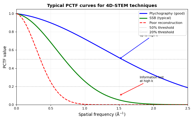
Ptychography typically maintains higher PCTF values to larger spatial frequencies because it uses multiple overlapping probe positions, providing redundant information. SSB imaging relies on center beam information and typically has a more limited frequency response. The spatial frequency where the PCTF drops below 0.5 or 0.2 defines your effective resolution limit.
Applications
The PCTF concept is used throughout 4D-STEM analysis:
Ptychography: Comparing reconstructed object phase to simulated ground truth
Single sideband imaging: Evaluating how well the phase is recovered from the center beam
Method comparison: Determining which reconstruction algorithm (ePIE, DM, ML) preserves more high frequency information
Parameter optimization: Finding optimal dose, overlap, or convergence angle by maximizing the PCTF
The PCTF provides a rigorous, quantitative way to evaluate reconstruction quality beyond visual inspection.
References