n=1 has 1s; n=2 has 2s, 2p; n=3 has 3s, 3p, 3d; n=4 has 4s, 4p, 4d, 4f; n=5 and beyond follow the same pattern as n=4. To determine the electron filling order, draw a table with rows for each principal quantum number n (from 1 at the top to 5 at the bottom). Start from 1s, go down, and then up diagonally to the right. Following these diagonals gives the correct order: 1s, 2s, 2p, 3s, 3p, 4s, 3d, 4p, 5s, 4d, 5p, 6s, etc.
Be able to have Fill Order from n=1 to 5
- Some rules: A half-filled or completely filled shell is more stable. Example: [Ar]4s^1 3d^5
What is a molecular orbital?
It is a linear combination of atomic orbitals.
What are the shapes and notations of molecular orbitals?
In the case of \(H_2\), \(\psi_{\sigma} = \psi_{1s}(r_A) + \psi_{1s}(r_B)\). The antibonding orbital is \(\psi_{\sigma^*} = \psi_{1s}(r_A) - \psi_{1s}(r_B)\). In terms of shape, the bonding orbital has two peaks with the middle region shared, so it’s greater than 0 in the y-axis. For the antibonding orbital, the two are opposite in direction, with a node (zero) in the middle.
What is the concept of bond order?
\(BO = 0.5 \times (\text{number of electrons in bonding orbitals} - \text{number in antibonding orbitals})\) It predicts the “number” of bonds.
How would you defined electronegativity?
The tendency of a given element to attract electrons when fomring a bond.
What are the four types of bonding in solids?
Metallic, covalent, ionic, and van der Waals.
What is valence?
Valence is the ability of an electron to combine wiht other elements. Its ability is determine by the outermost electrons.
What is hybridization?
Mixing of atomic orbitals with close energies.
What is coordination?
The number of nearest neighbors. Bonds with less directionality (ionic/metallic) tend to form with maximized coordination.
What is the concept of “shielding effect”?
Protons in the nucleus attract electrons inward. However, inner electrons repel outer electrons due to like charges. This repulsion partially cancels the nuclear attraction, so the effective pulling force from the nucleus (protons) on the outer electrons becomes weaker.
What is effective nuclear charge \((Z_{eff})\)? What is the trend of \(Z_{eff}\) across a period, a group, and as atomic number increases?
The effective nuclear charge is the net positive charge experienced by an electron in a multi-electron atom. Across a period (left to right), \(Z_{eff}\) increases because more protons are added while shielding does not increase as much. Down a group (top to bottom), \(Z_{eff}\) increases slightly, but the effect is less pronounced due to increased shielding from additional shells. As atomic number increases, \(Z_{eff}\) generally increases.
From the end of Period 2 to the start of Period 3, \(Z_{eff}\) drops suddenly. Why?
A new outer shell is added that is farther from the nucleus and more shielded by inner electrons, so the effective nuclear charge experienced by the outermost electrons decreases.
What is “atomic radius”? What is its trend?
Atomic radius is the distance from the nucleus to the outermost stable electron orbital. Across a period (left to right), atomic radius decreases because outer electrons experience a stronger pull toward the nucleus without the addition of a new shell. Down a group (top to bottom), atomic radius increases as a new electron shell is added.
Define ionization energy
The energy required to remove an electron from a gaseous atom or ion. \(IE = E(A^+_g) - E(A_g)\).
Define electron affinity
The energy change when a gas-phase atom gains an electron. \(EA = E(A^-_g) - E(A_g)\).
Describe the trend of ionization energy in the periodic table
Down a group, decrease. \(\uparrow\) shielding, \(\uparrow\) atomic radius → electrons easier to remove
Acorss a period, increase, \(\uparrow\)\(Z_{eff}\), \(\downarrow\) atomic radius \(\to\) electrons more tightly bound
How do you compute electronegativitiy?
The average between IE and EA.
What do you mean by “equivalent directions” in crystallography?
Two directions are equivalent if the crystal looks identical when viewed or translated along either one.
Why use 4 coordinate system for hexagonal?
In cubic systems, planes are described by three indices \((hkl)\), and the family \({100}\) includes three mutually perpendicular but equivalent planes: \((100)\), \((010)\), and \((001)\). In the hexagonal system, there are three equivalent axes in the basal plane: \(a_1\), \(a_2\), and \(a_3\). These are 120° apart and equal in length, related by a threefold rotational, so \({100}\) includes three distinct but equivalent planes: \((100)\), \((010)\), and \((1\bar{1}0)\). Because the usual \((hkl)\) notation cannot specify which in-plane axis (out of 3) is used, a four-index system \((hkil)\) is adopted to remove this ambiguity.
How do you convert from Miller to Miller-Bravais indices for hexagonal systems?
For hexagonal crystals, we convert from 3-index Miller notation to 4-index Miller-Bravais notation to explicitly show the symmetry of the three equivalent basal plane axes.
For directions\(\langle u'v'w' \rangle\) to \(\langle uvtw \rangle\):
\[u = \frac{1}{3}(2u' - v')\]
\[v = \frac{1}{3}(2v' - u')\]
\[t = -(u + v)\]
\[w = w'\]
The constraint \(t + u + v = 0\) ensures redundancy that makes the threefold symmetry explicit.
For planes\(\{h'k'l'\}\) to \(\{hkil\}\):
\[h = h'\]
\[k = k'\]
\[i = -(h + k)\]
\[l = l'\]
The third index \(i\) is determined by the constraint \(h + k + i = 0\), which follows from the relationship between the three basal plane reciprocal lattice vectors.
Note: The constraint that the sum of the first three Miller-Bravais indices equals zero (\(h + k + i = 0\) for planes, \(u + v + t = 0\) for directions) is required by international conventions and reflects the threefold symmetry of the hexagonal system.
Worked example for directions: Convert the direction \([2\bar{1}0]\) in Miller notation to Miller-Bravais notation.
What’s the structure factor and how is it relevant in modelling?
The structure factor, denoted as \(F(hkl)\), quantifies the amplitude and phase of X-ray scattering from a crystal lattice. It is calculated by summing the contributions of all atoms in the unit cell, taking into account their positions and scattering factors. The structure factor is crucial for predicting the intensity of diffracted beams in X-ray crystallography, as it directly influences the observed diffraction pattern.
What is the atomic scattering factor?
The atomic scattering factor \(f_j\) (also called form factor) represents how effectively an atom scatters X-rays. It depends on the electron density distribution around the nucleus and the scattering angle. Heavier atoms with more electrons scatter more strongly (\(f\) is larger), while lighter atoms scatter weakly. The scattering factor decreases with increasing scattering angle because constructive interference from the electron cloud becomes less effective at higher angles.
What is the structure factor equation?
\(F(hkl) = \sum_{j=1}^{N} f_j \exp\left[2\pi i (hx_j + ky_j + lz_j)\right]\) where \(f_j\) is the atomic scattering factor of atom \(j\), and \((x_j, y_j, z_j)\) are the fractional coordinates of atom \(j\) in the unit cell. \(h, k, l\) are the Miller indices of the reflecting plane.
How can you determine posiiton and intensty of diffraction peaks using structure factor?
The position of diffraction peaks is determined by the Miller indices \((hkl)\) and the geometry of the crystal lattice, while the intensity of each peak is proportional to the square of the magnitude of the structure factor: \(I(hkl) \propto |F(hkl)|^2\). By calculating the structure factor for different sets of Miller indices, one can predict both where diffraction peaks will occur and how intense they will be.
How did one determine the scattering factor?
The scattering factor \(f_j\) for an atom is determined experimentally by measuring the intensity of X-ray scattering as a function of the scattering angle. It depends on the type of atom and the angle of incidence, reflecting how effectively the atom scatters X-rays.
Can you give me a toy model of using BCC for a specific plane?
To calculate the structure factor for the (100) plane, we first identify the atomic positions in the BCC unit cell: (0,0,0) and (1/2,1/2,1/2). The structure factor is given by \(F(100) = f \left[ \exp(2\pi i (1*0 + 0*0 + 0*0)) + \exp(2\pi i (1*\frac{1}{2} + 0*\frac{1}{2} + 0*\frac{1}{2})) \right]\), and simplifying this yields \(F(100) = f [1 + \exp(\pi i)] = f [1 - 1] = 0\). This indicates that there is no diffraction peak for the (100) plane in a BCC structure. In BCC, reflections are forbidden when \(h+k+l\) is odd. The (110) reflection (\(h+k+l=2\), even) is allowed and is in fact the strongest BCC peak, with \(F(110) = 2f\).
Will (110) reflection show up in XRD for FCC?
For FCC (face-centered cubic), the basis consists of atoms at positions: \((0,0,0)\), \((0,\frac{1}{2},\frac{1}{2})\), \((\frac{1}{2},0,\frac{1}{2})\), \((\frac{1}{2},\frac{1}{2},0)\).
Calculate the structure factor for (110):
\[F_{110} = f \sum_{j} \exp[2\pi i(hx_j + ky_j + lz_j)]\]
Substitute \(h=1, k=1, l=0\) for each atomic position:
Therefore, \(F_{110} = 0\), which means no XRD peak appears for the (110) reflection in FCC. This is a systematic absence due to the face-centered structure.
General rule for FCC: Reflections (hkl) are allowed only when h, k, l are all even or all odd. Since (110) has mixed parity (two odd, one even), it is forbidden.
How does thermal expansion shift XRD peak positions?
When a material is heated, thermal expansion increases the lattice parameter, which changes the interplanar spacing and shifts diffraction peaks to lower angles (since \(d\) increases, \(\theta\) must decrease to satisfy Bragg’s law).
Example problem: An FCC material has lattice parameter \(a = 0.405\) nm at 298 K and expands to 500 K. Given the coefficient of linear thermal expansion \(\alpha_L = 24 \times 10^{-6}\) K⁻¹, find the angular shift in the (220) diffraction peak using X-rays with energy 8.04 keV.
Step 1: Calculate lattice parameter at elevated temperature
The negative shift indicates the peak moves to lower angles, which makes physical sense: thermal expansion increases \(d\), so a smaller \(\theta\) is needed to satisfy Bragg’s law.
Physical interpretation: As temperature increases, the lattice expands, planes get farther apart, and diffraction peaks shift to lower 2θ angles. This shift can be measured experimentally and used to determine thermal expansion coefficients or detect phase transitions.
How is interplanar spacing related to reciprocal lattice vectors?
The interplanar spacing \(d_{hkl}\) for a set of planes with Miller indices \((hkl)\) is inversely related to the magnitude of the reciprocal lattice vector \(\mathbf{G}_{hkl}\). Specifically:
This relationship connects real space (interplanar spacing) to reciprocal space (reciprocal lattice vectors).
How do you find interplanar spacing using the projection method?
There is an alternative geometric approach to find \(d_{hkl}\) using vector projection. The interplanar spacing is the perpendicular distance between adjacent parallel planes.
Step 1: Define the unit normal vector
The reciprocal lattice vector \(\mathbf{g}_{hkl}\) is perpendicular to the (hkl) planes (see proof-g-perpendicular-to-planes). The unit normal vector is:
Any vector \(\mathbf{t}\) that connects lattice points on adjacent planes can be used. For simplicity, we can use lattice vectors like \(\mathbf{a}\), \(\mathbf{b}\), or \(\mathbf{c}\), or any integer combination.
Step 3: Project onto the normal direction
The interplanar spacing is the component of \(\mathbf{t}\) along the normal direction:
Physical interpretation: Imagine standing perpendicular to a family of planes. The interplanar spacing is how far you must walk in that perpendicular direction to reach the next plane. If you take any path \(\mathbf{t}\) from one plane to the next, projecting it onto the perpendicular direction gives you \(d_{hkl}\).
Example: For a simple cubic lattice with lattice parameter \(a\), consider the (100) planes. The reciprocal lattice vector is \(\mathbf{g}_{100} = \frac{2\pi}{a}\hat{x}\), so \(|\mathbf{g}_{100}| = \frac{2\pi}{a}\). Using the translation vector \(\mathbf{t} = a\hat{x}\):
The metric tensor \(g\) encodes the geometry of the crystal lattice in the crystal frame. It contains all information about the lengths and angles between basis vectors \(\mathbf{a}\), \(\mathbf{b}\), \(\mathbf{c}\):
where \(a, b, c\) are lattice parameters and \(\alpha, \beta, \gamma\) are interaxial angles.
How does the metric tensor convert crystal to Cartesian coordinates?
In the crystal frame, a vector with coefficients \((u, v, w)\) means \(\mathbf{r} = u\mathbf{a} + v\mathbf{b} + w\mathbf{c}\). To find its length in real space, we compute:
\[\begin{split}|\mathbf{r}|^2 = \begin{pmatrix} u & v & w \end{pmatrix}
\begin{pmatrix}
a^2 & ab\cos\gamma & ac\cos\beta \\
ba\cos\gamma & b^2 & bc\cos\alpha \\
ca\cos\beta & cb\cos\alpha & c^2
\end{pmatrix}
\begin{pmatrix} u \\ v \\ w \end{pmatrix}
= \begin{pmatrix} u & v & w \end{pmatrix} g \begin{pmatrix} u \\ v \\ w \end{pmatrix}\end{split}\]
The metric tensor \(g\) thus converts crystal frame coefficients to real space distances without explicitly constructing Cartesian coordinates.
Why is the metric tensor useful?
The metric tensor allows us to compute distances, angles, and volumes directly in the crystal frame. For example, the angle \(\theta\) between two crystallographic directions can be calculated without converting to Cartesian coordinates.
Setting up the problem: Consider two directions in the crystal:
Direction 1: \([u_1 \, v_1 \, w_1]\) corresponds to the real space vector \(\mathbf{r}_1 = u_1\mathbf{a} + v_1\mathbf{b} + w_1\mathbf{c}\)
Direction 2: \([u_2 \, v_2 \, w_2]\) corresponds to the real space vector \(\mathbf{r}_2 = u_2\mathbf{a} + v_2\mathbf{b} + w_2\mathbf{c}\)
Computing the angle: The angle between these vectors is given by:
\(|\mathbf{r}_1|^2 = \mathbf{r}_1 \cdot \mathbf{r}_1 = \mathbf{u}_1^T g \mathbf{u}_1\), so \(|\mathbf{r}_1| = \sqrt{\mathbf{u}_1^T g \mathbf{u}_1}\)
\(|\mathbf{r}_2|^2 = \mathbf{r}_2 \cdot \mathbf{r}_2 = \mathbf{u}_2^T g \mathbf{u}_2\), so \(|\mathbf{r}_2| = \sqrt{\mathbf{u}_2^T g \mathbf{u}_2}\)
Final formula: Combining these gives:
\[\boxed{\cos\theta = \frac{\mathbf{u}_1^T g \mathbf{u}_2}{\sqrt{\mathbf{u}_1^T g \mathbf{u}_1} \sqrt{\mathbf{u}_2^T g \mathbf{u}_2}}}\]
where \(\mathbf{u}_1 = (u_1, v_1, w_1)^T\) and \(\mathbf{u}_2 = (u_2, v_2, w_2)^T\) are the column vectors of crystal frame coefficients. This is particularly useful for non-orthogonal crystal systems where direct Cartesian conversion would be cumbersome.
What are the metric tensor structures for the 7 crystal systems?
Each crystal system has a specific form of the metric tensor based on its symmetry constraints. The general triclinic form simplifies progressively as symmetry increases:
The reciprocal metric tensor \(g^*\) is defined for the reciprocal lattice, just as the direct metric tensor \(g\) is defined for the direct lattice. It encodes the geometry of the reciprocal lattice vectors \(\mathbf{a}^*, \mathbf{b}^*, \mathbf{c}^*\):
where \(a^*, b^*, c^*\) are reciprocal lattice parameters and \(\alpha^*, \beta^*, \gamma^*\) are reciprocal interaxial angles.
How is the reciprocal metric tensor related to the direct metric tensor?
The reciprocal metric tensor matrix is the inverse of the direct metric tensor matrix (see What is the metric tensor? for the direct metric tensor). If we denote the direct metric tensor as \(G\) and the reciprocal metric tensor as \(G^*\), then:
\[G^* = G^{-1}\]
This means that \(G \cdot G^* = I\), where \(I\) is the identity matrix. This inverse relationship is fundamental to crystallography and connects real space to reciprocal space. Note that in component form, the direct metric tensor elements are \(g_{ij} = \mathbf{a}_i \cdot \mathbf{a}_j\) and the reciprocal metric tensor elements are \(g^*_{ij} = \mathbf{a}^*_i \cdot \mathbf{a}^*_j\).
What are the reciprocal metric tensor structures for different crystal systems?
The reciprocal metric tensors follow the same symmetry patterns as the direct metric tensors. Here are examples for key systems:
Hexagonal reciprocal metric tensor:
For a hexagonal lattice with direct metric tensor \(g_{\text{hexagonal}}\):
How do you calculate the length of a reciprocal lattice vector?
A reciprocal lattice vector with Miller indices \((hkl)\) in the crystal frame corresponds to \(\mathbf{g} = h\mathbf{a}^* + k\mathbf{b}^* + l\mathbf{c}^*\) (see reciprocal-lattice-definition). The length \(|\mathbf{g}|\) represents the actual physical length in Cartesian space (in units like Å-1), which is what we measure in diffraction experiments. Just like in direct space (see What is the metric tensor?), we use the reciprocal metric tensor to compute this length directly from the crystal frame coefficients \((hkl)\).
In matrix form using the reciprocal metric tensor \(G^*\):
\[\begin{split}|\mathbf{g}|^2 = \begin{pmatrix} h & k & l \end{pmatrix} G^* \begin{pmatrix} h \\ k \\ l \end{pmatrix}\end{split}\]
Therefore:
\[\begin{split}|\mathbf{g}| = \sqrt{\begin{pmatrix} h & k & l \end{pmatrix} G^* \begin{pmatrix} h \\ k \\ l \end{pmatrix}}\end{split}\]
This is exactly analogous to computing distances in direct space using the direct metric tensor, but applied to reciprocal space.
How do you calculate the angle between two reciprocal lattice vectors?
For two reciprocal lattice vectors \(\mathbf{g}_1 = h_1\mathbf{a}^* + k_1\mathbf{b}^* + l_1\mathbf{c}^*\) and \(\mathbf{g}_2 = h_2\mathbf{a}^* + k_2\mathbf{b}^* + l_2\mathbf{c}^*\), the angle \(\theta\) between them is:
This formula is completely parallel to the direct space case (see What is the metric tensor? for computing angles between directions), but uses the reciprocal metric tensor\(G^*\) and Miller indices \((hkl)\) instead of direction indices \([uvw]\).
How do you transform vectors between direct and reciprocal space?
Consider a physical vector \(\mathbf{p}\) in space. This vector exists independently of whatever coordinate system we choose to describe it. We can express this same vector using either direct space basis vectors \(\{\mathbf{a}, \mathbf{b}, \mathbf{c}\}\) or reciprocal space basis vectors \(\{\mathbf{a}^*, \mathbf{b}^*, \mathbf{c}^*\}\):
The key insight is that \(\mathbf{a}_i \cdot \mathbf{a}_j^* = \delta_{ij}\), which means:
\(\mathbf{a}_1 \cdot \mathbf{a}_1^* = 1\), but \(\mathbf{a}_1 \cdot \mathbf{a}_2^* = 0\) and \(\mathbf{a}_1 \cdot \mathbf{a}_3^* = 0\)
\(\mathbf{a}_2 \cdot \mathbf{a}_2^* = 1\), but \(\mathbf{a}_2 \cdot \mathbf{a}_1^* = 0\) and \(\mathbf{a}_2 \cdot \mathbf{a}_3^* = 0\)
\(\mathbf{a}_3 \cdot \mathbf{a}_3^* = 1\), but \(\mathbf{a}_3 \cdot \mathbf{a}_1^* = 0\) and \(\mathbf{a}_3 \cdot \mathbf{a}_2^* = 0\)
This is the defining property of reciprocal lattice vectors (see reciprocal-lattice-definition). Now look at the right side of our equation. We have a sum over index \(j\):
Because of orthogonality, only one term survives: the one where \(j = m\). All other dot products are zero. For example, if \(m = 1\) (we’re dotting with \(\mathbf{a}_1\)), then:
We haven’t done anything to the left side yet, so we can factor it:
\[p_i (\mathbf{a}_i \cdot \mathbf{a}_m) = p_m^*\]
Step 5: Recognize the metric tensor
The term \(\mathbf{a}_i \cdot \mathbf{a}_m\) is exactly the definition of the metric tensor element \(g_{im}\) (the dot product of basis vectors). Therefore:
\[\boxed{p_i g_{im} = p_m^*}\]
Result: To convert from direct to reciprocal components, multiply by the metric tensor: \(p_m^* = p_i g_{im}\).
Concrete example with hexagonal lattice:
Consider a hexagonal lattice with \(a = 3\) Å, \(c = 5\) Å (\(\gamma = 120°\)). The direct metric tensor is:
Suppose we have a vector with direct space components \(\mathbf{p} = (1, 1, 0)\) in the crystal frame (meaning \(\mathbf{p} = 1 \cdot \mathbf{a}_1 + 1 \cdot \mathbf{a}_2 + 0 \cdot \mathbf{a}_3\)). What are its reciprocal space components?
Using \(p_m^* = p_i g_{im}\), we compute each component by taking the dot product of \(\mathbf{p}\) with each row of \(G\):
So the reciprocal space components are \(\mathbf{p}^* = (4.5, 4.5, 0)\), meaning \(\mathbf{p} = 4.5 \cdot \mathbf{a}_1^* + 4.5 \cdot \mathbf{a}_2^* + 0 \cdot \mathbf{a}_3^*\).
We can verify this works in reverse. Using \(p_i = p_m^* g_{mi}^*\), multiply \(\mathbf{p}^* = (4.5, 4.5, 0)\) by each row of \(G^*\):
Result: The reciprocal basis vectors \(\mathbf{a}_m^*\) can be obtained by multiplying the direct basis vectors \(\mathbf{a}_i\) by the reciprocal metric tensor \(g_{mi}^*\).
What this means: If you want to find what \(\mathbf{a}^*\) looks like in terms of \(\{\mathbf{a}, \mathbf{b}, \mathbf{c}\}\), you multiply \(\{\mathbf{a}, \mathbf{b}, \mathbf{c}\}\) by the reciprocal metric tensor. The rows of \(G^*\) give you the components of the reciprocal basis vectors expressed in the direct basis.
The reverse transformation:
By the same reasoning, you can show:
\[\boxed{\mathbf{a}_m = g_{mi} \mathbf{a}_i^*}\]
The rows of \(G\) give you the components of the direct basis vectors expressed in the reciprocal basis.
How does this prove that the metric tensors are inverses?
We can now prove that \(G^* = G^{-1}\) using what we just derived.
Step 1: Start with the fundamental orthogonality condition
From the definition of reciprocal space (see reciprocal-lattice-definition), we know:
But \(\mathbf{a}_i \cdot \mathbf{a}_k\) is exactly the definition of the metric tensor \(g_{ik}\):
\[g_{mi}^* g_{ik} = \delta_{mk}\]
Step 5: Recognize this as matrix multiplication
The equation \(g_{mi}^* g_{ik} = \delta_{mk}\) uses Einstein summation notation (repeated indices are summed). Let’s unpack what this means step by step.
Understanding the sum: For a specific choice of \(m\) and \(k\), we sum over the repeated index \(i\):
To obtain the reciprocal metric tensor: compute the inverse of the metric tensor
To determine the reciprocal basis vectors: pre-multiply the direct space basis vectors by the reciprocal metric tensor
What is a zone axis?
A zone axis \([uvw]\) is a crystallographic direction along which the electron beam travels. It defines the viewing direction through the crystal. All lattice planes \((hkl)\) that contain this direction satisfy the zone axis equation:
\[hu + kv + lw = 0\]
This equation determines which planes are “edge-on” when viewing along \([uvw]\). For example, consider the [001] zone axis (\(u=0, v=0, w=1\)):
In diffraction, only reflections from planes in the zone contribute to the pattern, which is why different zone axes show completely different diffraction patterns.
Derivation from reciprocal lattice definition:
Start with the definition of reciprocal lattice vectors. For a crystal with primitive lattice vectors \(\mathbf{a}_1, \mathbf{a}_2, \mathbf{a}_3\), the reciprocal lattice vectors are:
These satisfy the orthogonality condition: \(\mathbf{a}_i \cdot \mathbf{b}_j = 2\pi \delta_{ij}\).
How do we derive the reciprocal lattice vector formulas for 2D?
For a 2D crystal with primitive lattice vectors \(\mathbf{a}_1\) and \(\mathbf{a}_2\), the reciprocal lattice vectors \(\mathbf{b}_1\) and \(\mathbf{b}_2\) must satisfy the orthogonality condition \(\mathbf{a}_i \cdot \mathbf{b}_j = \delta_{ij}\).
Step 1: Start with the requirement for \(\mathbf{b}_1\)
We need \(\mathbf{b}_1\) perpendicular to \(\mathbf{a}_2\) (so \(\mathbf{a}_2 \cdot \mathbf{b}_1 = 0\)) and normalized such that \(\mathbf{a}_1 \cdot \mathbf{b}_1 = 1\).
Step 2: Construct perpendicular vector in 2D
In 2D, if \(\mathbf{a}_2 = (a_{2x}, a_{2y})\), then a perpendicular vector is \((-a_{2y}, a_{2x})\) (rotate by 90°). We can write:
\[\mathbf{b}_1 = C \cdot \text{perpendicular to } \mathbf{a}_2\]
More formally, for vectors in the xy-plane, the perpendicular direction can be obtained using the cross product with \(\hat{z}\):
\[\mathbf{b}_1 = C (\hat{z} \times \mathbf{a}_2)\]
The scalar triple product \(\mathbf{u} \cdot (\mathbf{v} \times \mathbf{w})\) is cyclic, meaning you can rotate the order of vectors without changing its value:
Using this cyclic property, \(\mathbf{a}_1 \cdot (\hat{z} \times \mathbf{a}_2) = \hat{z} \cdot (\mathbf{a}_2 \times \mathbf{a}_1)\). Since swapping \(\mathbf{a}_1\) and \(\mathbf{a}_2\) flips the sign:
The term \(\hat{z} \cdot (\mathbf{a}_1 \times \mathbf{a}_2)\) is the area \(A\) of the 2D unit cell.
Note
Geometric intuition: The cross product \(\mathbf{a}_1 \times \mathbf{a}_2\) gives an “area vector” pointing perpendicular to the plane. Its magnitude equals the area, and its direction indicates the orientation (up or down). When we compute \(A = \hat{z} \cdot (\mathbf{a}_1 \times \mathbf{a}_2)\), we are projecting this area vector onto the \(+z\) direction to find how much of it points along \(+z\). For 2D lattices in the xy-plane, this projection gives the signed area.
Therefore, the reciprocal lattice vectors are \(\mathbf{b}_1 = \left(\frac{4}{9}, -\frac{1}{9}\right)\) and \(\mathbf{b}_2 = \left(\frac{1}{9}, \frac{2}{9}\right)\).
How do we derive the reciprocal lattice vector formulas for 3D?
For the 3D case, we use the orthogonality condition \(\mathbf{a}_i \cdot \mathbf{b}_j = 2\pi \delta_{ij}\), where \(\delta_{ij}\) is the Kronecker delta (equals 1 when \(i = j\), and 0 when \(i \neq j\)).
Note
Note on the 2π factor: We include the \(2\pi\) factor here for completeness and to match the physics convention commonly used in solid-state physics and electron diffraction. This factor will cancel out when we calculate observable quantities like interplanar spacings, as we will see later. The crystallography convention (without \(2\pi\)) is also valid and commonly used in X-ray crystallography.
Step 1: Start with the requirement for \(\mathbf{b}_1\)
We need \(\mathbf{b}_1\) to satisfy the orthogonality conditions with all three lattice vectors. This means \(\mathbf{b}_1\) must be perpendicular to both \(\mathbf{a}_2\) and \(\mathbf{a}_3\) (so their dot products equal zero), but have a specific projection along \(\mathbf{a}_1\) (so \(\mathbf{a}_1 \cdot \mathbf{b}_1 = 2\pi\)).
Step 2: Use the cross product to ensure perpendicularity
The cross product \(\mathbf{a}_2 \times \mathbf{a}_3\) gives a vector perpendicular to both \(\mathbf{a}_2\) and \(\mathbf{a}_3\). So we can write:
\[\mathbf{b}_1 = C (\mathbf{a}_2 \times \mathbf{a}_3)\]
where \(C\) is a constant to be determined.
Step 3: Apply the normalization condition
We need \(\mathbf{a}_1 \cdot \mathbf{b}_1 = 2\pi\). Substitute our expression for \(\mathbf{b}_1\):
The same procedure applies to \(\mathbf{b}_2\) and \(\mathbf{b}_3\) by cyclic permutation. The denominator \(V = \mathbf{a}_1 \cdot (\mathbf{a}_2 \times \mathbf{a}_3)\) is the volume of the unit cell.
How do we go from reciprocal lattice vectors back to real space lattice vectors?
If you know the reciprocal lattice vectors \(\mathbf{b}_1, \mathbf{b}_2, \mathbf{b}_3\), you can recover the real space lattice vectors \(\mathbf{a}_1, \mathbf{a}_2, \mathbf{a}_3\) using the same formulas, but with the roles reversed.
Key insight: The reciprocal of the reciprocal lattice is the original lattice.
Step 1: Write the inverse formulas
Since \(\mathbf{b}_i \cdot \mathbf{a}_j = 2\pi \delta_{ij}\), the real space vectors satisfy the same orthogonality condition with the reciprocal vectors. Therefore:
Using the relationship \(V^* = (2\pi)^3/V\) and the fact that the construction is symmetric, this simplifies to \(2\pi\), confirming the orthogonality condition.
How do we find reciprocal lattice vectors for orthogonal systems?
For an orthorhombic cell where the lattice vectors are mutually perpendicular (orthogonal), the reciprocal lattice vector formulas simplify dramatically.
Key insight: For orthogonal systems, each reciprocal lattice vector is parallel to its corresponding real space vector, and the magnitude is simply the inverse of the real space lattice parameter. The reciprocal lattice is also orthogonal.
A general reciprocal lattice vector for planes with Miller indices \((hkl)\) is:
The key insight is that \(\mathbf{G}_{hkl}\) is perpendicular to the \((hkl)\) planes.
Proof: Why is \(\mathbf{G}_{hkl}\) perpendicular to (hkl) planes?
This can be proven by showing that \(\mathbf{G}_{hkl}\) is perpendicular to any vector lying within an \((hkl)\) plane.
Step 1: Identify vectors in the plane
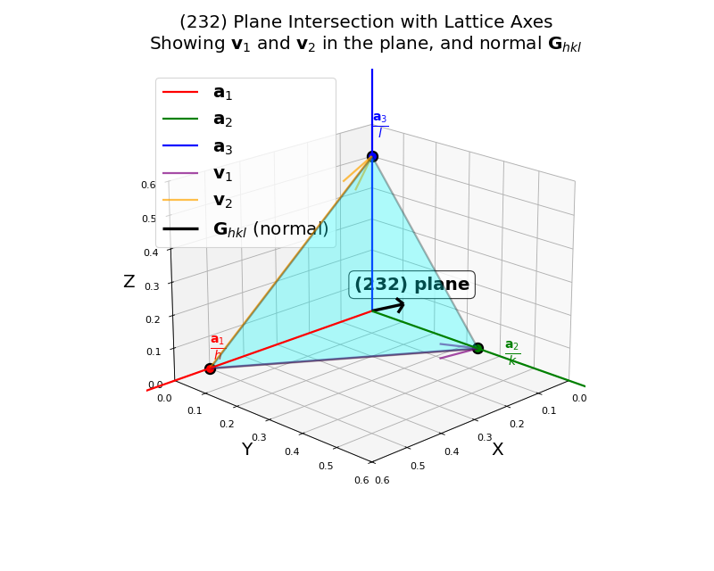
The \((hkl)\) plane nearest to the origin intersects the lattice axes at:
\(\frac{\mathbf{a}_1}{h}\) along the \(\mathbf{a}_1\) direction
\(\frac{\mathbf{a}_2}{k}\) along the \(\mathbf{a}_2\) direction
\(\frac{\mathbf{a}_3}{l}\) along the \(\mathbf{a}_3\) direction
The (232) plane intersecting the lattice axes at \(\frac{\mathbf{a}_1}{2}\), \(\frac{\mathbf{a}_2}{3}\), and \(\frac{\mathbf{a}_3}{2}\). The vectors \(\mathbf{v}_1\) (purple) and \(\mathbf{v}_2\) (orange) lie within the plane. The reciprocal lattice vector \(\mathbf{G}_{hkl}\) (black) is perpendicular to the plane.
Any two vectors connecting these intercept points lie in the \((hkl)\) plane. For example:
Since \(\mathbf{G}_{hkl}\) is perpendicular to two independent vectors in the plane, it must be perpendicular to the entire \((hkl)\) plane.
Relationship to interplanar spacing:
The interplanar spacing \(d_{hkl}\) is the perpendicular distance between adjacent parallel planes.
Why introduce vector R? We know how to calculate \(\mathbf{G}_{hkl}\) (the reciprocal lattice vector) from the real space lattice vectors. But how do we connect this to the real-space quantity \(d_{hkl}\) that we can measure experimentally? The key insight is to consider any lattice vector \(\mathbf{R}\) that connects equivalent points on adjacent planes. Since we can write \(\mathbf{R}\) in terms of the lattice vectors \(\mathbf{a}_1, \mathbf{a}_2, \mathbf{a}_3\), and we know the orthogonality condition \(\mathbf{a}_i \cdot \mathbf{b}_j = 2\pi \delta_{ij}\), we can calculate \(\mathbf{R} \cdot \mathbf{G}_{hkl}\) and relate it to \(d_{hkl}\).
Consider a lattice vector \(\mathbf{R}\) that connects equivalent points on adjacent \((hkl)\) planes. Important: \(\mathbf{R}\) is generally not perpendicular to the planes and \(|\mathbf{R}| \neq d_{hkl}\). The smallest such vector can be written as:
where \(n_1, n_2, n_3\) are integers chosen such that \(\mathbf{R}\) connects adjacent planes.
Why the fractions n/h, n/k, n/l? Remember that the (hkl) plane closest to the origin intersects the axes at \(\frac{\mathbf{a}_1}{h}\), \(\frac{\mathbf{a}_2}{k}\), and \(\frac{\mathbf{a}_3}{l}\). This is the definition of Miller indices. To reach the next parallel plane, we need to move by integer multiples of these fractional intercepts. For example, if we start at a point on the first plane and want to reach an equivalent point on the second plane, we might move by \(\frac{1}{h}\mathbf{a}_1\) (choosing \(n_1 = 1, n_2 = 0, n_3 = 0\)). The h, k, l denominators ensure that \(\mathbf{R}\) connects lattice points that lie exactly on adjacent (hkl) planes.
The interplanar spacing is the projection of \(\mathbf{R}\) onto the direction normal to the planes, which is along \(\mathbf{G}_{hkl}\):
Why this projection formula? The vector \(\mathbf{R}\) connects points on adjacent planes, but it lies at an angle to the plane normal. To find the perpendicular distance between planes (the interplanar spacing), we project \(\mathbf{R}\) onto the direction normal to the planes. Since \(\mathbf{G}_{hkl}\) is perpendicular to the planes, the unit normal is \(\hat{n} = \frac{\mathbf{G}_{hkl}}{|\mathbf{G}_{hkl}|}\). The projection gives the perpendicular component:
\[= \frac{n_1}{h} \cdot h \cdot 2\pi + \frac{n_2}{k} \cdot k \cdot 2\pi + \frac{n_3}{l} \cdot l \cdot 2\pi = 2\pi(n_1 + n_2 + n_3)\]
For adjacent planes, choose \(\mathbf{R}\) such that \(n_1 + n_2 + n_3 = 1\) (e.g., \(n_1 = 1, n_2 = 0, n_3 = 0\)), giving:
\[d_{hkl} = \frac{2\pi}{|\mathbf{G}_{hkl}|}\]
Why\(n_1 + n_2 + n_3 = 1\)for adjacent planes? The vector \(\mathbf{R} = \frac{1}{h}\mathbf{a}_1\) already connects a point on one (hkl) plane to the next parallel plane, because the planes are defined by their fractional intercepts along the crystal axes. Any choice with \(n_1 + n_2 + n_3 = 1\) gives the same projection \(d_{hkl}\) onto the plane normal. Higher values of \(n_1 + n_2 + n_3\) correspond to spacing between non-adjacent planes.
In cubic crystals with lattice parameter \(a\), the reciprocal lattice vectors simplify significantly. The reciprocal lattice is also cubic with parameter \(\frac{2\pi}{a}\). For Miller indices \((hkl)\):
This equation describes the Ewald sphere construction in reciprocal space.
Note
In crystallography, the reciprocal lattice is often defined without the \(2\pi\) factor, using \(|\mathbf{k}| = \frac{1}{\lambda}\) and \(G = \frac{1}{d}\) instead. This gives \(G = \frac{2}{\lambda}\sin(\theta)\). The physics convention (used above with \(2\pi\)) is common in solid-state physics and electron diffraction, while the crystallography convention (without \(2\pi\)) is typical in X-ray crystallography.
Ewald circle construction (2D cross-section along [001] zone axis) for a cubic crystal with lattice parameter a = 0.5 nm and incident wavelength λ = 0.193 nm. The cyan circle represents the Ewald circle with radius |k| = 2π/λ. Blue dots are reciprocal lattice points in the (h,k,0) plane, and red stars indicate points where the Laue diffraction condition \(\mathbf{G} = \mathbf{k}_{out} - \mathbf{k}_{in}\) is satisfied. The incident wave vector \(\mathbf{k}_{in}\) (red), example diffracted wave vector \(\mathbf{k}_{out}\) (green), and corresponding reciprocal lattice vector \(\mathbf{G}\) (orange) are shown.
What is the relationship between Ewald’s sphere and Bragg’s law?
Ewald’s sphere construction in reciprocal space is equivalent to Bragg’s law in real space. Here’s how they connect using the crystallography convention (without \(2\pi\)):
Step 1: Start with the Ewald sphere result
From the derivation above (using crystallography convention):
\[G = \frac{2}{\lambda}\sin(\theta)\]
Step 2: Use the reciprocal lattice definition
The magnitude of a reciprocal lattice vector is:
\[G = \frac{1}{d}\]
where \(d\) is the interplanar spacing.
Step 3: Equate both expressions
\[\frac{1}{d} = \frac{2}{\lambda}\sin(\theta)\]
Step 4: Rearrange to get Bragg’s law
\[\lambda = 2d\sin(\theta)\]
For higher order reflections, this becomes:
\[n\lambda = 2d\sin(\theta)\]
where \(n\) is an integer.
Conclusion: This shows that Ewald’s sphere construction (in reciprocal space) and Bragg’s law (in real space) are mathematically equivalent descriptions of the diffraction condition.
What is the Bragg’s condition?
\(n\lambda = 2d\sin\theta\) where \(d\) is the interplanar spacing, \(\theta\) is the angle of incidence, and \(n\) is an integer representing the order of reflection.
What’s the relationship bewteen Ewarld’s sphere and Laue condition?
The Laue condition states that diffraction occurs when the difference between the incident and diffracted wave vectors equals a reciprocal lattice vector: \(\mathbf{G} = \mathbf{k}_{out} - \mathbf{k}_{in}\). Ewald’s sphere visually represents this condition in reciprocal space, where the tips of the wave vectors lie on the surface of a sphere with radius \(|\mathbf{k}| = \frac{2\pi}{\lambda}\). When a reciprocal lattice point intersects the Ewald sphere, the Laue condition is satisfied, indicating that diffraction will occur.
What’s the relationship between Laue condition and Bragg’s law?
Both describe the conditions for diffraction. The Laue condition is expressed in terms of wave vectors in reciprocal space, while Bragg’s law is formulated in real space using interplanar spacing and angles. They are mathematically equivalent, as shown by deriving Bragg’s law from the Laue condition.
Apply normal and shear strain components to a 2D unit cell and watch how the lattice deforms. See how the strain tensor maps to physical distortions like extension, compression, and shear.
![Ewald circle construction in reciprocal space, [001] zone axis](../_images/plot_ewald_sphere.png)