Phase contrast physics
Understanding electron wave phase
Electron microscopy faces a fundamental challenge: we cannot directly measure phase, yet phase often carries the most important information about our samples. This is known as the phase problem.
How phase is lost
Here is what actually happens in the microscope:
Incident wave enters sample:
\[\psi_{\text{in}}(x,y) = e^{ik_0 z}\]Sample modifies the wave (object transmission function):
\[\psi_{\text{exit}}(x,y) = \psi_{\text{in}}(x,y) \cdot O(x,y) = \psi_{\text{in}}(x,y) \cdot A(x,y) e^{i\phi(x,y)}\]The object \(O(x,y) = A(x,y) e^{i\phi(x,y)}\) encodes both amplitude changes \(A\) (scattering, absorption) and phase shifts \(\phi\) (potential).
Exit wave propagates to detector:
\[I(k_x, k_y) = |\mathcal{F}\{\psi_{\text{exit}}(x,y)\}|^2\]We measure the diffraction pattern intensity in reciprocal space (k-space).
Phase is lost: The detector measures \(|\cdot|^2\), which destroys the complex phase \(e^{i\phi}\). We lose the information connecting \(\phi(x,y)\) to the potential \(V(x,y)\).
Phase retrieval is the inverse problem: Given measured intensities \(I(k_x,k_y)\), reconstruct the phase \(\phi(x,y)\) (and thus the potential \(V\) through \(\phi = \sigma V\)).
Why we need phase
Phase and intensity provide complementary information:
Intensity (what we measure): Shows where electrons scatter strongly. Scales as ~:math:Z^2 (atomic number squared). Heavy elements (high Z) show strong contrast.
Phase (what we want): Shows electromagnetic field distributions. Scales as \(\int V \, dz\) (integrated potential). Even light elements create substantial phase shifts.
This distinction matters for light-element imaging. Consider a biological sample made of carbon, nitrogen, and oxygen (\(Z = 6, 7, 8\)):
Weak scattering: Low Z → low intensity contrast (~:math:Z^2) → barely visible in conventional TEM
Strong potentials: Atoms still create electrostatic potentials → substantial phase accumulation (\(\phi \propto \int V \, dz\))
A thin biological sample may be nearly invisible in intensity images but creates large, measurable phase shifts. Phase retrieval is essential for imaging soft matter and light-element structures.
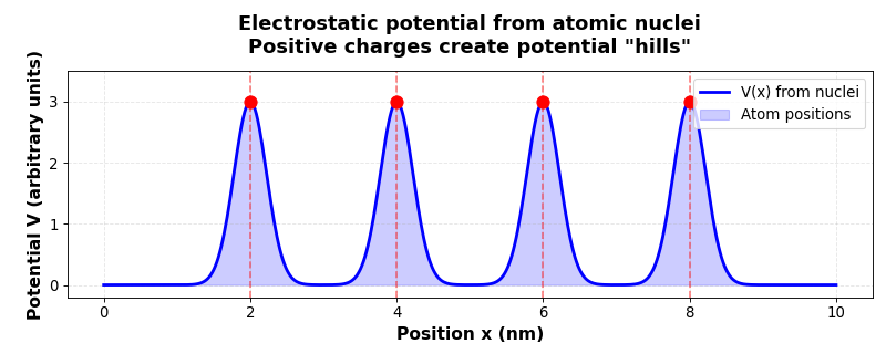
The electrostatic potential forms “hills” at atomic positions. Negative electrons are attracted toward these peaks (positive nuclei), causing deflection and phase accumulation.
Physics of phase shift
When an electron wave interacts with a sample, it undergoes two distinct changes:
Amplitude changes \(A(x,y)\): Electrons are absorbed or scattered away
Easy to measure directly
Shows where electrons interact strongly
Scales as ~:math:Z^2 (atomic number squared)
Heavy elements give strong contrast
Phase shifts \(\phi(x,y)\): The wave’s oscillation is delayed by the sample’s potential
Cannot measure directly
Contains crucial information about fields and potentials
Scales linearly with potential
Even light elements create substantial shifts
Important
The phase problem arises because our detectors can only measure intensity \(|\psi|^2 = |A|^2\), which tells us about amplitude but completely erases phase information.
Mathematical foundations
The phase retrieval problem can be expressed mathematically as:
where:
\(I(x,y)\) is the measured intensity
\(\psi(x,y)\) is the complex wave function
\(A(x,y)\) is the amplitude
We want to recover \(\phi(x,y)\) where \(\psi(x,y) = A(x,y)e^{i\phi(x,y)}\)
The measurement challenge
When an electron wave passes through a sample, it undergoes two types of changes:
Amplitude changes \(A(x,y)\): electrons are absorbed or scattered away
Phase shifts \(\phi(x,y)\): the wave’s oscillation is delayed by the sample’s electrostatic potential
The exit wave (the wave leaving the sample) carries both amplitude and phase information. However, detectors can only measure intensity = \(|\psi_{\text{exit}}|^2\), which contains amplitude information but completely erases the phase. This is problematic because the exit wave’s phase \(\phi(x,y)\) directly encodes the sample’s electrostatic potential \(V(x,y)\).
How phase shifts occur
Note
Key assumptions in this phase shift model:
The following summarizes the main approximations used to derive the phase object approximation \(\phi = \sigma V\).
- Non-relativistic quantum mechanics
What it means: Use Schrödinger equation (not Dirac equation) to describe electron wavefunction
Valid when: Works well for typical TEM energies (80-300 keV). We still account for relativistic effects on electron mass and wavelength
Note: See separate quantum mechanics page for detailed discussion of relativistic corrections
- Elastic scattering
What it means: No energy transfer to sample
Valid when: Dominant at small angles. Inelastic scattering increases with thickness and Z
- Single scattering
What it means: Electron interacts with potential only once
Valid when: Thin samples (< 10-50 nm). Multiple scattering increases with thickness and Z
- Paraxial approximation
What it means: Electron travels primarily along beam direction; transverse momentum changes small
Valid when: \(|\partial A/\partial z| \ll k_0 |A|\). Valid for small angles (< few mrad)
- Projection approximation
What it means: Neglect transverse diffraction: \(\nabla_{\perp}^2 A \approx 0\)
Valid when: Sample thickness ≪ transverse feature size. Valid for t < 20-50 nm
- Weak-phase object
What it means: Phase shift small: \(|\sigma V| \ll 1\), allowing \(e^{i\sigma V} \approx 1 + i\sigma V\)
Valid when: Thin samples with low Z. Breaks down when \(\sigma V > 0.5\) radians
- Electrostatic approximation
What it means: Magnetic interactions negligible
Valid when: Valid except for ferromagnets. Magnetic phase \(\sim 10^{-3}\) of electrostatic
When these assumptions break down:
Thick samples: Multiple scattering, breakdown of projection approximation, strong phase shifts
Heavy elements: Large phase shifts violate weak-phase approximation, increased inelastic scattering
Large scattering angles: Paraxial approximation fails, need full dynamical diffraction theory
Crystalline samples at zone axis: Dynamical diffraction (Bragg scattering) dominates over kinematic scattering
Note
Notation used in this section:
\(V(x,y,z)\): Electrostatic potential (volts) at position (x,y,z)
\(V(x,y) = \int V(x,y,z) dz\): Projected potential (integrated through thickness)
\(\phi(x,y)\): Phase shift (radians) accumulated by electron wave
\(\phi = \sigma V\): Phase object approximation (see phase-object-approximation)
\(\sigma = \pi/(E\lambda)\): Interaction constant (see Derivation of interaction constant)
\(E\): Electron kinetic energy (keV)
\(\lambda = h/p\): Electron de Broglie wavelength
\(q = 1.602 \times 10^{-19}\) C: Elementary charge magnitude (positive)
Electron charge: \(-q\) (negative)
\(k_0 = \sqrt{2mE}/\hbar = 2\pi/\lambda\): Incident wave vector
\(\nabla_{\perp} = (\partial/\partial x, \partial/\partial y)\): Transverse gradient operator
\(\nabla_{\perp} \phi = \sigma \nabla_{\perp} V\): Phase gradient relationship (see Phase gradient derivation)
\(E_{\text{total}} = E_{\text{kinetic}} - qV\): Energy conservation (see energy-conservation-electrons)
\(\hbar = h/(2\pi)\): Reduced Planck constant
\(m\): Electron mass
Electrostatic potential in the sample
The electrostatic potential \(V(x,y,z)\) describes the influence that charged particles (nuclei and electrons) in the sample exert on other charged particles passing through. It represents the potential energy per unit charge at each point in space.
In a material, positively charged atomic nuclei create regions of elevated (more positive) potential. We can think of the potential landscape as having “peaks” or “hills” centered at each atomic position, with the potential decreasing as you move away from the nuclei.
How electrons respond to the potential landscape
A positive test charge placed on top of a potential hill would naturally “roll down” toward lower potential (away from the positively charged nuclei), moving from high potential to low potential to minimize its potential energy. Conversely, a negative charge (like an electron) experiences the opposite behavior—it is attracted up the potential hills, toward the positively charged nuclei at the peaks.
When an electron beam passes through this potential landscape, each electron experiences a force because it carries a negative charge. Electrons are attracted toward the positively charged nuclei (the potential peaks), causing the electron wave to be deflected and to accumulate phase as it propagates through the sample.
The projected potential
The projected potential \(V(x,y)\) is the integral through the sample thickness:
This projection represents the total potential “seen” by an electron traveling along the beam direction (z-axis). When an electron wave passes through a sample, it accumulates a phase shift proportional to this projected potential:
where \(\sigma = \pi/(E\lambda)\) is the interaction constant, \(E\) is electron energy, and \(\lambda\) is wavelength.
The phase object approximation
In the phase object approximation (also called the projection approximation, valid for thin samples), the transmitted electron wave can be written as:
where \(\sigma = \pi/(E\lambda)\) and \(V(x,y) = \int V(x,y,z) dz\) is the projected potential.
Derivation of interaction constant
To derive the interaction constant \(\sigma\), we solve the Schrödinger equation for a fast electron passing through a thin sample.
Starting point: Time-independent Schrödinger equation
For an electron in a potential \(V(\mathbf{r})\):
Step 1: Separate longitudinal and transverse coordinates
Write \(\psi(\mathbf{r}) = \psi(x,y,z)\) and assume the electron propagates primarily in the z-direction with high energy E. Use the ansatz:
where \(k_0 = \sqrt{2mE}/\hbar\) is the incident wave vector and \(A(x,y,z)\) is a slowly varying envelope function.
Understanding k₀
The incident wave vector \(k_0 = \sqrt{2mE}/\hbar\) comes from the relationship between energy and momentum in quantum mechanics. For a free electron:
For a free electron (V = 0) traveling in the z-direction, the wavefunction is a plane wave:
\[\psi = e^{ik_0 z}\]The energy eigenvalue equation gives:
\[-\frac{\hbar^2}{2m} \frac{d^2 \psi}{dz^2} = E \psi\]Substituting \(\psi = e^{ik_0 z}\):
\[-\frac{\hbar^2}{2m}(ik_0)^2 e^{ik_0 z} = E e^{ik_0 z}\]\[\frac{\hbar^2 k_0^2}{2m} = E\]Therefore:
\[k_0 = \sqrt{\frac{2mE}{\hbar^2}} = \frac{\sqrt{2mE}}{\hbar}\]This relates the wave vector to the electron’s kinetic energy. Using \(p = \hbar k_0\), this is equivalent to the classical relation \(E = p^2/(2m)\).
Step 2: Apply paraxial approximation
Since the electron has high energy and the sample is thin, \(A(x,y,z)\) varies slowly with z compared to \(e^{ik_0 z}\). We can approximate \(\partial^2 A/\partial z^2 \ll k_0 \partial A/\partial z\).
Full derivation
Computing the Laplacian
Start with \(\psi = A(x,y,z) e^{ik_0 z}\). We need to compute \(\nabla^2 \psi\):
1. Longitudinal derivatives
First derivative with respect to z:
Second derivative with respect to z:
2. Transverse derivatives
Since \(e^{ik_0 z}\) is constant with respect to x and y:
3. Complete Laplacian
The full Laplacian is the sum of all second derivatives:
where \(\nabla_{\perp}^2 = \frac{\partial^2}{\partial x^2} + \frac{\partial^2}{\partial y^2}\) is the transverse Laplacian.
Paraxial approximation
For fast electrons (high \(k_0\)), the envelope function \(A(x,y,z)\) varies slowly with z:
This leads to the paraxial wave equation:
This equation describes how the electron wave evolves as it propagates through the sample’s potential.
\[\nabla^2 \psi = \left[\nabla_{\perp}^2 A + \frac{\partial^2 A}{\partial z^2} + 2ik_0 \frac{\partial A}{\partial z} - k_0^2 A\right] e^{ik_0 z}\]where \(\nabla_{\perp}^2 = \partial^2/\partial x^2 + \partial^2/\partial y^2\).
Substitute into Schrödinger equation \(-\frac{\hbar^2}{2m}\nabla^2\psi + V\psi = E\psi\):
\[-\frac{\hbar^2}{2m}\left[\nabla_{\perp}^2 A + \frac{\partial^2 A}{\partial z^2} + 2ik_0 \frac{\partial A}{\partial z} - k_0^2 A\right] e^{ik_0 z} + V A e^{ik_0 z} = E A e^{ik_0 z}\]Divide by \(e^{ik_0 z}\):
\[-\frac{\hbar^2}{2m}\left[\nabla_{\perp}^2 A + \frac{\partial^2 A}{\partial z^2} + 2ik_0 \frac{\partial A}{\partial z} - k_0^2 A\right] + VA = EA\]Use \(k_0^2 = 2mE/\hbar^2\) to cancel terms:
The \(-k_0^2 A\) term becomes:
\[-\frac{\hbar^2}{2m}(-k_0^2 A) = \frac{\hbar^2 k_0^2}{2m} A = \frac{\hbar^2}{2m} \cdot \frac{2mE}{\hbar^2} A = EA\]This exactly cancels the \(EA\) on the right side:
\[-\frac{\hbar^2}{2m}\left[\nabla_{\perp}^2 A + \frac{\partial^2 A}{\partial z^2} + 2ik_0 \frac{\partial A}{\partial z}\right] + VA = 0\]Neglect \(\partial^2 A/\partial z^2\) (paraxial approximation):
\[-\frac{\hbar^2}{2m}\left[\nabla_{\perp}^2 A + 2ik_0 \frac{\partial A}{\partial z}\right] + VA = 0\]Rearrange:
\[2ik_0 \frac{\partial A}{\partial z} + \nabla_{\perp}^2 A + \frac{2m}{\hbar^2} VA = 0\]This gives the paraxial wave equation:
\[2ik_0 \frac{\partial A}{\partial z} + \nabla_{\perp}^2 A + \frac{2m}{\hbar^2} V(x,y,z) A = 0\]Step 3: Projection approximation (thin sample)
For a thin sample, we can neglect transverse diffraction during propagation (\(\nabla_{\perp}^2 A \approx 0\)). This gives:
\[\frac{\partial A}{\partial z} = -\frac{im}{\hbar^2 k_0} V(x,y,z) A\]Step 4: Integrate through sample
Integrating from z = 0 (entrance) to z = t (exit):
\[A(x,y,t) = A(x,y,0) \exp\left[-\frac{im}{\hbar^2 k_0} \int_0^t V(x,y,z) dz\right]\]Recall the full wavefunction: \(\psi = A(x,y,z) e^{ik_0 z}\), so at the exit:
\[\psi_{\text{exit}} = A(x,y,0) \exp\left[-\frac{im}{\hbar^2 k_0} \int_0^t V(x,y,z) dz\right] e^{ik_0 t}\]Combine the exponentials:
\[\psi_{\text{exit}} = A(x,y,0) \exp\left[ik_0 t - \frac{im}{\hbar^2 k_0} \int_0^t V(x,y,z) dz\right]\]The phase shift \(\phi(x,y)\) is the change from the incident phase \(k_0 t\):
\[\phi(x,y) = -\frac{m}{\hbar^2 k_0} \int_0^t V(x,y,z) dz = -\frac{m}{\hbar^2 k_0} V(x,y)\]Step 5: Express in terms of electron wavelength
Using \(k_0 = 2\pi/\lambda\) and \(E = \hbar^2 k_0^2/(2m)\), we can rewrite:
\[\boxed{\phi(x,y) = -\frac{m}{\hbar^2 k_0} V(x,y) = \frac{\pi}{E\lambda} V(x,y) = \sigma V(x,y)}\]where \(\sigma = \pi/(E\lambda)\) is the interaction constant and \(V(x,y) = \int V(x,y,z) dz\) is the projected potential.
Key insights:
Phase shift proportional to projected potential
Higher potential → larger phase accumulation
Lower energy electrons (larger λ) → more sensitive to potential
Linear relationship enables quantitative analysis
The electron wave accumulates phase as it travels through the sample. Regions with higher potential (near atoms) cause a larger phase shift compared to regions with lower potential (vacuum or between atoms). This phase modulation encodes information about the atomic structure.
For very thin samples where \(\sigma V(x,y) \ll 1\), we can use a first-order Taylor expansion (the weak-phase object approximation):
This linearizes the relationship between the potential and the exit wave, simplifying phase retrieval algorithms. Most DPC and ptychography reconstructions assume this weak-phase regime.
Phase gradient derivation
From the phase object approximation, \(\phi(x,y) = \sigma V(x,y)\). Taking the gradient in the transverse plane:
where \(\nabla_{\perp} = (\partial/\partial x, \partial/\partial y)\).
Electric field integration
The transverse electric field integrated along the beam path:
Momentum transfer
The momentum transfer to the electron:
Final relationship
Therefore:
Note
The deflection angle \(\theta \approx \Delta p_{\perp}/p_z\) is directly related to the phase gradient.
Connection to electron deflection
The gradient of the phase tells us the deflection angle:
Since the electric field is \(\mathbf{E} = -\nabla V\), electrons (being negatively charged) are deflected in the direction of \(+\nabla V\), which is opposite to the electric field direction. They are attracted toward the positively charged nuclei (the potential peaks).
By measuring the center of mass (CoM) shift of the diffraction pattern at each probe position, we can determine the local deflection angle, and from that, reconstruct the phase gradient \(\nabla \phi\). Integrating this gradient gives us the phase \(\phi(x,y)\), and thus the projected potential \(V(x,y)\). This is the principle behind Differential Phase Contrast (DPC) imaging.
The physics of phase accumulation
In quantum mechanics, an electron wavefunction \(\psi = A e^{i\phi(t)}\) evolves according to its total energy:
Time evolution derivation
This fundamental relationship comes from the time-dependent Schrödinger equation. Here’s the derivation:
Starting point
The time-dependent Schrödinger equation:
where \(\hat{H}\) is the Hamiltonian operator (total energy operator) and \(\hbar\) is the reduced Planck constant.
Step 1: Assume wavefunction form
Write the wavefunction as:
where \(A\) is the amplitude (constant) and \(\phi(t)\) is the time-dependent phase.
Step 2: Take time derivative
Step 3: Substitute into Schrödinger equation
Step 4: For energy eigenstate
For a state with definite energy \(E_{\text{total}}\), the Hamiltonian acts as:
Step 5: Final result
Substituting and dividing both sides by \(\psi\):
Physical interpretation: Higher energy → faster phase oscillation. The negative sign means the phase decreases with time (rotates clockwise in the complex plane).
When the electron passes through a region with electrostatic potential \(V(z)\), its total energy becomes:
where \(q = 1.602 \times 10^{-19}\) C is the elementary charge magnitude (positive). The electron carries charge \(-q\) (negative). Important: The total energy \(E_{\text{total}}\) is conserved—it remains constant throughout the sample. However, the electron’s kinetic energy temporarily changes as it interacts with the potential. Near a positively charged nucleus (where \(V > 0\), a potential “hill”), the negatively charged electron is attracted and speeds up, gaining kinetic energy (the \(-qV\) term becomes more negative, so \(E_{\text{kinetic}}\) increases). Far from nuclei (between atoms), it slows down. Think of it like a ball rolling through a landscape of hills and valleys—the ball speeds up going downhill and slows down going uphill, but its total energy stays constant.
This change in kinetic energy corresponds to a change in the electron’s wavelength (via de Broglie relation \(\lambda = h/p\)). Since the wavefunction’s phase advance depends on how many wavelengths fit into a distance, different regions accumulate phase at different rates. As the electron propagates through thickness \(dz\) in time \(dt = dz/v\), the accumulated phase shift is:
Integrating through the sample thickness and using the de Broglie relation \(\lambda = h/p\) with relativistic expressions for electron energy and momentum yields the interaction constant \(\sigma = \pi/(E\lambda)\).
Understanding the interaction constant
The factor \(\sigma = \pi/(E\lambda)\) converts electrostatic potential (volts) to phase shift (radians). It depends on the microscope’s operating parameters:
E is the accelerating voltage: 80 kV, 200 kV, or 300 kV → electrons gain 80 keV, 200 keV, or 300 keV of kinetic energy
\(\lambda\) is the electron wavelength: higher energy → shorter wavelength (300 keV → \(\lambda \approx 0.002\) nm, comparable to atomic spacings)
\(\sigma\) has units (keV·nm)⁻¹, making \(\phi = \sigma V\) dimensionless (radians)
Example: For 300 keV electrons, \(\sigma \approx 0.729\) rad/(V·nm). A single carbon atom (creating ~1 V·nm of integrated potential) shifts the phase by ~0.7 radians.
Key insight: Lower-energy electrons (larger \(\lambda\), smaller E) have larger \(\sigma\) → more sensitive to potentials → accumulate more phase for the same sample. This is why low-voltage electron microscopy enhances phase contrast for light elements.