Image processing

Affine transformations

What is an affine transformation?

An affine transformation maps point \((x, y)\) to \((x', y')\) via matrix multiplication:

\[\begin{split}\begin{bmatrix} x' \\ y' \\ 1 \end{bmatrix} = \begin{bmatrix} a & b & t_x \\ c & d & t_y \\ 0 & 0 & 1 \end{bmatrix} \begin{bmatrix} x \\ y \\ 1 \end{bmatrix}\end{split}\]

This expands to \(x' = ax + by + t_x\) and \(y' = cx + dy + t_y\). The 2×3 matrix \(\begin{bmatrix} a & b & t_x \\ c & d & t_y \end{bmatrix}\) defines the transformation.

What are common transformation examples?

Translation (shift by \(t_x, t_y\)):

\[\begin{split}\begin{bmatrix} 1 & 0 & t_x \\ 0 & 1 & t_y \end{bmatrix}\end{split}\]

Example: shift right 50 pixels, down 30 pixels:

\[\begin{split}\begin{bmatrix} 1 & 0 & 50 \\ 0 & 1 & 30 \end{bmatrix}\end{split}\]

Scaling (by factors \(s_x, s_y\)):

\[\begin{split}\begin{bmatrix} s_x & 0 & 0 \\ 0 & s_y & 0 \end{bmatrix}\end{split}\]

Example: double width, half height:

\[\begin{split}\begin{bmatrix} 2 & 0 & 0 \\ 0 & 0.5 & 0 \end{bmatrix}\end{split}\]

Rotation (by angle \(\theta\) counterclockwise):

\[\begin{split}\begin{bmatrix} \cos\theta & -\sin\theta & 0 \\ \sin\theta & \cos\theta & 0 \end{bmatrix}\end{split}\]

Example: rotate 45° around origin:

\[\begin{split}\begin{bmatrix} 0.707 & -0.707 & 0 \\ 0.707 & 0.707 & 0 \end{bmatrix}\end{split}\]

Shearing (horizontal by factor \(k\)):

\[\begin{split}\begin{bmatrix} 1 & k & 0 \\ 0 & 1 & 0 \end{bmatrix}\end{split}\]

Example: horizontal shear with k=0.5:

\[\begin{split}\begin{bmatrix} 1 & 0.5 & 0 \\ 0 & 1 & 0 \end{bmatrix}\end{split}\]

What does “linear” mean mathematically?

A transformation \(T\) is linear if it satisfies:

Additivity: \(T(\mathbf{a} + \mathbf{b}) = T(\mathbf{a}) + T(\mathbf{b})\)
Homogeneity: \(T(c\mathbf{a}) = cT(\mathbf{a})\)

Translation fails this test. For \(T(x, y) = (x + 5, y + 3)\):

\[T((1, 2) + (3, 4)) = T(4, 6) = (9, 9)\]

but

\[T(1, 2) + T(3, 4) = (6, 5) + (8, 7) = (14, 12)\]

Therefore, translation is not linear.

Why is it called “affine” and not “linear”?

Translation breaks linearity because \(f(0) \neq 0\) when \(t_x\) or \(t_y\) are non-zero. “Affine” (from Latin affinis meaning “related”) means linear plus a constant shift.

Properties preserved:

Parallel lines remain parallel
Ratios of distances along the same line are preserved (collinearity)
Midpoints are preserved (a line segment’s midpoint remains its midpoint, though coordinates change)

Properties not preserved:

Origin is shifted
Angles change (except rotation and reflection)
Distances change (except rotation and translation)
Ratios of distances between different directions change (e.g., scaling stretches width but not height)
Areas change (except rotation and translation)

Visualization of affine transformations:

(Source code, png, hires.png, pdf)

../_images/plot_affine_transformations.png

The figure demonstrates various affine transformations and their properties:

Row 1: Different transformation types (translation, rotation, scaling, shearing) applied to a rectangle with parallel lines and midpoints marked
Row 2: More transformations including horizontal shear, vertical shear, reflection, and combined operations
Row 3: Property demonstrations showing that parallel lines stay parallel (blue dashed lines remain parallel after shearing), ratios along the same line are preserved (collinear points maintain ratio 1.00 even after 2x scaling), midpoints are preserved (the midpoint of a line segment remains the midpoint after rotation, though its absolute coordinates change), but angles change (90° becomes 117° after shearing)

What are the advantages of affine transformations?

Compact: Only 6 parameters define any affine transformation
Composable: Chaining transformations reduces to matrix multiplication
Invertible: Easy to compute inverse transformation

Applications:

Image registration (aligning photos from different angles)
Lens distortion correction
Medical imaging (CT and MRI alignment)
Computer graphics (sprite transformations)
Document scanning (correcting perspective skew)

What can’t affine transformations do?

Curved distortions like lens barrel or pincushion effects require:

Perspective transformations (projective)
Polynomial warping
Radial distortion models

Image alignment

Template matching

What is template matching?

Template matching locates a small reference image (template) within a larger image by computing similarity at each position.

Why use template matching in electron microscopy?

Drift correction: During long acquisitions, thermal expansion, mechanical vibrations, and stage instabilities cause specimen shifts between frames. Template matching tracks a distinctive feature (atomic column, nanoparticle, or edge) across frames to measure displacement.

Two correction approaches:

Post-acquisition: Measure drift vectors and computationally realign frames
Real-time feedback: Actively adjust stage position during acquisition

Without drift correction, multi-frame averaging blurs atomic features.

How does template matching work?

For a 512×512 image and 10×10 template:

Place template at position \((x, y)\)
Compute similarity score between template and image region
Slide template to next position
Repeat for all ~250,000 positions
Similarity map peaks indicate template locations

Cross-correlation

How is cross-correlation used in template matching?

Cross-correlation computes the similarity score at each position by multiplying corresponding pixels and summing results.

What is cross-correlation?

Cross-correlation uses two coordinate systems:

Global coordinates \((x,y)\): Template position in the large image
Local coordinates \((u,v)\): Pixel indices within the template

For a template of size \(M \times N\), the cross-correlation at position \((x,y)\) is:

\[C(x,y) = \sum_{u=0}^{M-1} \sum_{v=0}^{N-1} T(u,v) \cdot I(x+u, y+v)\]

Example: Template \(\begin{bmatrix} 100 & 150 \\ 120 & 180 \end{bmatrix}\) with image region \(\begin{bmatrix} 95 & 145 \\ 125 & 175 \end{bmatrix}\):

\[C = (100)(95) + (150)(145) + (120)(125) + (180)(175) = 77{,}750\]

Why does higher cross-correlation mean better match?

When bright pixels align with bright pixels and dark with dark, each multiplication produces a large positive number. High sum indicates similarity.

What is the problem with raw cross-correlation?

Brightness variations dominate the score. A featureless bright region can outscore a perfect pattern match in a darker area.

Example: Template [10, 20, 30]

Match against itself: \(C = 10^2 + 20^2 + 30^2 = 1400\)
Match against bright patch [100, 100, 100]: \(C = 10(100) + 20(100) + 30(100) = 6000\)

The uniform brightness wins by 4×, despite capturing none of the pattern.

Why use normalized cross-correlation?

Normalized cross-correlation (NCC) measures pattern shape rather than absolute brightness by subtracting means and dividing by standard deviations:

\[\text{NCC}(x,y) = \frac{\sum_{u,v} [T(u,v) - \bar{T}][I(x+u,y+v) - \bar{I}]}{\sqrt{\sum_{u,v}[T(u,v) - \bar{T}]^2 \sum_{u,v}[I(x+u,y+v) - \bar{I}]^2}}\]

where \(\bar{T}\) is the template’s mean intensity and \(\bar{I}\) is the image region’s mean.

Output range: -1 (inverted pattern) to +1 (perfect match)

Robust to:

Lighting changes
Contrast variations
Detector gain differences

Fourier-based alignment

What is Fourier-based alignment?

Fourier-based alignment detects image shifts by working in frequency space. The Fourier shift theorem states: translation in real space becomes a phase shift in frequency space.

Why is this important for beam tilt correction?

In beam tilt corrected STEM (tcBF-STEM), each detector pixel corresponds to a different beam tilt angle. By reciprocity, this creates multiple shifted views of the same sample. Fourier-based alignment provides the speed and accuracy needed to align thousands of these shifted images.

How does the Fourier shift theorem work?

Translating an image by \((\Delta x, \Delta y)\) multiplies its Fourier transform by a phase factor:

\[\mathcal{F}\{f(x - \Delta x, y - \Delta y)\} = e^{-2\pi i(k_x \Delta x + k_y \Delta y)} \mathcal{F}\{f(x,y)\}\]

where \(k_x\) and \(k_y\) are spatial frequencies. The magnitude remains unchanged—only the phase shifts.

How do you apply the Fourier shift theorem?

To shift an image by \((\Delta x, \Delta y) = (2.5, 1.3)\) pixels:

Compute FFT: Call np.fft.fft2() to get complex array \(F[i,j] = a + bi\)
Calculate phase shift for each frequency \((k_x, k_y)\):

\[\theta = -2\pi(k_x \Delta x + k_y \Delta y)\]

At frequency (0.1, 0.2):

\[\theta = -2\pi(0.1 \times 2.5 + 0.2 \times 1.3) = -3.20 \text{ rad}\]
Convert to complex number:

\[e^{i\theta} = \cos(-3.20) + i\sin(-3.20) = -0.9899 - 0.1411i\]
Multiply Fourier coefficient: For \(F[i,j] = 3.62 + 3.73i\):

\[(3.62 + 3.73i)(-0.9899 - 0.1411i) = -3.057 - 4.203i\]
Verify magnitude preservation:
- Before: \(\sqrt{3.62^2 + 3.73^2} = 5.20\)
- After: \(\sqrt{3.057^2 + 4.203^2} = 5.20\) ✓
Inverse FFT: np.fft.ifft2() reconstructs the shifted image

Repeat for all 262,144 elements (512×512 image). The shift never moves pixels directly—it modifies phases in frequency space.

What is the computational cost of real-space shifting?

For a 1024×1024 image with known shift:

Integer shifts (e.g., exactly 10 pixels):

Copy each pixel to new position: ~1 million operations

Sub-pixel shifts (e.g., 10.5 pixels):

Requires interpolation between neighboring pixels
Linear interpolation: 4 operations per pixel
Bicubic interpolation: 10 operations per pixel
Total: ~10 million operations

How does Fourier shifting compare?

Computational cost:

Two FFTs + phase multiplication: ~21 million operations
Independent of shift amount

When real-space wins:

Integer shifts: 1M operations (21× faster than Fourier)
Sub-pixel shifts: 10M operations (2× faster than Fourier)

Fourier advantages:

Simpler implementation (no coordinate transformation logic)
No edge handling required
Sub-pixel precision natural from phase
Both methods produce equivalent quality

Why use Fourier-based shifts for unknown shifts?

The advantage emerges when measuring drift between two images where the shift amount is unknown.

Brute force real-space search:

Testing all possible integer shifts from -50 to +50 pixels in both directions:

Shift candidates: 101 × 101 = 10,201 positions
Each trial: shift image (~1M ops) + compute similarity (~1M ops) = 2M ops
Total: ~20 billion operations

Phase correlation in Fourier space:

Three FFTs: ~31 million operations
Produces 2D map where peak directly reveals shift
All 10,000+ candidates evaluated simultaneously
Speedup: 600×

Sub-pixel precision comparison:

Real-space with 10 sub-pixel positions per integer shift:

Search space: 1,010 × 1,010 = 1,020,100 positions
Each sub-pixel shift requires interpolation (~10M ops)
Total: ~10 trillion operations

Fourier phase correlation:

Coarse shift: 31M operations
Sub-pixel refinement: ~1M operations
Speedup: 30,000×

Phase correlation in Fourier space

What is phase correlation?

Phase correlation finds the shift between two images by comparing phases in frequency space.

Given reference image \(I_1\) and shifted image \(I_2\):

Compute Fourier transforms \(F_1\) and \(F_2\)
Calculate cross-power spectrum:

\[R = \frac{F_1 \cdot F_2^*}{|F_1 \cdot F_2^*|}\]
Inverse Fourier transform of \(R\) produces a sharp peak at \((\Delta x, \Delta y)\)

The peak position directly reveals the shift.

How does this differ from template matching?

Template matching:

Scans every position
Complexity: \(O(N^2M^2)\) for \(N \times N\) image and \(M \times M\) template
Can find rotations and complex patterns

Phase correlation:

Uses FFT
Complexity: \(O(N^2 \log N)\)
Handles entire image at once
Only for translations
Superior speed and sub-pixel accuracy for shifts

Subpixel image shifting

What is subpixel image shifting?

Subpixel shifting moves an image by a non-integer number of pixels (e.g., shift by 2.7 pixels right, 1.3 pixels down). This is essential for:

Image registration and alignment
Motion correction in microscopy
Super-resolution reconstruction
Drift correction in time series

Since digital images exist on a discrete pixel grid, shifting by non-integer amounts requires interpolation to estimate values at new positions.

The interpolation problem

Consider shifting an image 1.5 pixels to the right. The new pixel at position \(x\) needs the value that was originally at position \(x - 1.5\). But \(x - 1.5\) lies between two pixels, so we must interpolate.

Key challenge: How do we estimate the intensity at a fractional pixel position?

Bilinear interpolation

Bilinear interpolation estimates the intensity at position \((x, y)\) using the four nearest pixels in a 2×2 neighborhood.

Step 1: Find the four surrounding pixels

For fractional position \((x, y)\):

\((x_0, y_0)\) = floor coordinates (pixel below-left)
\((x_1, y_1)\) = \((x_0 + 1, y_0 + 1)\) (pixel above-right)

The four corners are: \((x_0, y_0)\), \((x_1, y_0)\), \((x_0, y_1)\), \((x_1, y_1)\)

Step 2: Compute fractional offsets

\[\alpha = x - x_0 \quad \text{(horizontal fraction, 0 to 1)}\]

\[\beta = y - y_0 \quad \text{(vertical fraction, 0 to 1)}\]

Step 3: Interpolate horizontally first

Along the bottom edge \(y = y_0\):

\[I_{\text{bottom}} = (1 - \alpha) \cdot I(x_0, y_0) + \alpha \cdot I(x_1, y_0)\]

Along the top edge \(y = y_1\):

\[I_{\text{top}} = (1 - \alpha) \cdot I(x_0, y_1) + \alpha \cdot I(x_1, y_1)\]

Step 4: Interpolate vertically

\[I(x, y) = (1 - \beta) \cdot I_{\text{bottom}} + \beta \cdot I_{\text{top}}\]

Expanding:

\[I(x, y) = (1-\alpha)(1-\beta) I(x_0,y_0) + \alpha(1-\beta) I(x_1,y_0) + (1-\alpha)\beta I(x_0,y_1) + \alpha\beta I(x_1,y_1)\]

This is a weighted average where weights decrease linearly with distance from \((x, y)\).

Numerical example

Suppose we want the intensity at position \((2.3, 1.7)\) given a 2×2 neighborhood:

\[\begin{split}\begin{bmatrix} 100 & 150 \\ 120 & 180 \end{bmatrix}\end{split}\]

where pixel \((2, 1)\) has intensity 100 (bottom-left).

Step 1: Fractional offsets: \(\alpha = 0.3\), \(\beta = 0.7\)

Step 2: Horizontal interpolation

Bottom: \(I_{\text{bottom}} = 0.7 \times 100 + 0.3 \times 150 = 70 + 45 = 115\)

Top: \(I_{\text{top}} = 0.7 \times 120 + 0.3 \times 180 = 84 + 54 = 138\)

Step 3: Vertical interpolation

\(I(2.3, 1.7) = 0.3 \times 115 + 0.7 \times 138 = 34.5 + 96.6 = 131.1\)

The interpolated intensity is 131.1, smoothly blending the four neighbors.

Implementation with PyTorch grid_sample

PyTorch’s grid_sample function performs efficient bilinear interpolation for entire images using GPU acceleration.

The coordinate transformation:

Given a shift \((\Delta x, \Delta y)\):

Create sampling grid: For each output pixel at \((i, j)\), compute where to sample from the input image:

\[x_{\text{sample}} = j - \Delta x\]

\[y_{\text{sample}} = i - \Delta y\]
Normalize to [-1, 1]: grid_sample expects coordinates in normalized space where -1 is the left/top edge and +1 is the right/bottom edge:

\[x_{\text{norm}} = 2 \cdot \frac{x_{\text{sample}}}{W - 1} - 1\]

\[y_{\text{norm}} = 2 \cdot \frac{y_{\text{sample}}}{H - 1} - 1\]
Sample with bilinear interpolation: grid_sample reads from the input image at the normalized coordinates, automatically performing bilinear interpolation.

Why normalize to [-1, 1]?

This convention allows grid_sample to work with images of any size. The normalization maps:

Top-left corner \((0, 0)\) → \((-1, -1)\)

Bottom-right corner \((H-1, W-1)\) → \((1, 1)\)

Center pixel → \((0, 0)\)

Positions outside [-1, 1] fall outside the image boundary (handled by padding_mode).

Example: Shifting by (0.5, -0.3) pixels

To shift right by 0.5 and up by 0.3:

import torch

H, W = 256, 256
image = torch.rand(H, W)  # Random test image
shift_x, shift_y = 0.5, -0.3

# Create meshgrid
y = torch.arange(H, dtype=torch.float32)
x = torch.arange(W, dtype=torch.float32)
yy, xx = torch.meshgrid(y, x, indexing='ij')

# Apply inverse shift (sample from original positions)
yy_shifted = yy - shift_y  # Sample from y + 0.3
xx_shifted = xx - shift_x  # Sample from x - 0.5

# Normalize to [-1, 1]
yy_norm = 2.0 * yy_shifted / (H - 1) - 1.0
xx_norm = 2.0 * xx_shifted / (W - 1) - 1.0

# Create grid (1, H, W, 2)
grid = torch.stack([xx_norm, yy_norm], dim=-1).unsqueeze(0)

# Apply grid_sample
image_4d = image.unsqueeze(0).unsqueeze(0)  # (1, 1, H, W)
shifted = torch.nn.functional.grid_sample(
    image_4d, grid,
    mode='bilinear',           # Bilinear interpolation
    padding_mode='zeros',      # Pad with zeros outside boundary
    align_corners=True         # Align corner pixels to [-1, 1]
)

shifted_image = shifted.squeeze()  # Back to (H, W)

The output shifted_image is the input shifted by (0.5, -0.3) pixels with smooth interpolation.

Why the inverse shift?

The grid specifies where to read from in the input image, not where to write to. To shift the image right by 0.5 pixels, each output pixel must read from 0.5 pixels to the left in the input. This is the inverse mapping:

\[\text{output}[i, j] = \text{input}[i - \Delta y, j - \Delta x]\]

This “pull” approach (read from source) is more efficient than “push” (write to destination) because it avoids conflicts when multiple source pixels map to the same destination.

Comparison with other interpolation methods

Nearest-neighbor:

Fastest (no computation)
Blocky artifacts
Use for: categorical data (labels, segmentation masks)

Bilinear:

Fast and smooth
Blurs sharp edges slightly
Use for: natural images, intensity data

Bicubic:

Uses 4×4 neighborhood (16 pixels)
Sharper edges than bilinear
Higher computational cost
Use for: high-quality image scaling, super-resolution

Fourier shift theorem:

Shift in real space = phase ramp in Fourier space
Perfect for periodic signals
Circular boundary conditions (wraparound)
Use for: crystallography, phase correlation

For most microscopy applications, bilinear interpolation provides an excellent balance of speed and quality.

Common pitfalls

1. Forgetting the inverse mapping: To shift right, sample from the left!

2. Coordinate system mismatch: grid_sample expects (x, y) order in the last dimension, but meshgrid with indexing=’ij’ produces (y, x). Must stack as [xx, yy], not [yy, xx].

3. Off-by-one errors: With align_corners=True, coordinates range from corner to corner. With align_corners=False, coordinates reference pixel centers. Be consistent!

4. Boundary handling: padding_mode=’zeros’ pads with black, padding_mode=’border’ replicates edge pixels, padding_mode=’reflection’ mirrors. Choose based on physical expectations.

Image noise models

Understanding noise sources

In scientific imaging (electron microscopy, astronomy, medical imaging), noise is unavoidable due to fundamental physical limitations:

Dose limitations: Too much radiation damages samples
Fast imaging: Short exposure times capture dynamics but reduce signal
Low-light conditions: Weak signals produce poor signal-to-noise ratios

The noise characteristics determine what information can be extracted and what denoising strategies are effective.

Shot noise (Poisson)

Physical origin

Shot noise arises from the discrete, random nature of particle detection. Each photon or electron arrival is an independent event following Poisson statistics.

Mathematical model

For a pixel with true intensity \(u\), the observed count \(f\) follows:

\[f \sim \text{Poisson}(\lambda \cdot u)\]

where \(\lambda\) is the photon count scale (dose).

Key properties

Variance equals mean: \(\sigma^2 = \lambda \cdot u\)
Signal-to-noise ratio: \(\text{SNR} = \sqrt{\lambda \cdot u}\)
Brighter pixels have better relative SNR
Low-dose imaging (small \(\lambda\)) increases relative noise

Example: Visualizing Poisson noise

Consider a simple test image with three intensity levels:

(Source code, png, hires.png, pdf)

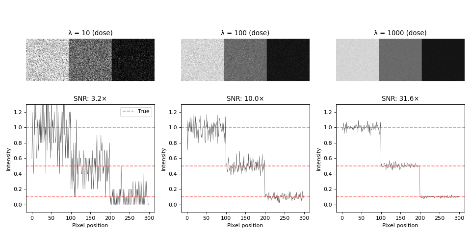
Observations:

Low dose (λ=10): Severe graininess, dim region barely visible, SNR≈3×
Medium dose (λ=100): Moderate noise, all regions distinguishable, SNR≈10×
High dose (λ=1000): Smooth appearance, clear boundaries, SNR≈32×
Bright regions (u=1.0) have large absolute noise but good relative SNR
Dim regions (u=0.1) have small absolute noise but poor relative SNR

The dim region at λ=10 has ~30% noise, making quantitative analysis difficult. Increasing dose to λ=1000 reduces noise to ~3%.

Thermal and readout noise

Thermal noise (Gaussian): Electronic components generate random voltage fluctuations with Gaussian distribution:

\[f(x,y) = u(x,y) + \mathcal{N}(0, \sigma^2)\]

Unlike Poisson noise, thermal noise is signal-independent: \(\sigma\) is constant across the image.

Readout noise: Analog-to-digital conversion introduces quantization errors and electronic readout noise, also typically Gaussian.

For modern detectors, shot noise usually dominates in low-light conditions, while thermal/readout noise becomes significant in bright conditions or with poor electronics.

Correlated temporal noise

The noise models above assume each pixel and each frame is independent (uncorrelated). In reality, imaging systems often exhibit temporal correlations where noise patterns persist across consecutive frames. These correlated noise sources are critical for time-series imaging:

Why independent noise is insufficient

Simple Poisson or Gaussian noise assumes each measurement is independent:

\[I_t(x,y) \sim \text{Poisson}(\lambda \cdot u(x,y))\]

Each frame at time \(t\) is independent of frame \(t-1\). This breaks down when:

The sample drifts during imaging
Mechanical vibrations affect the microscope
Detector artifacts appear in bursts
Motion blur from fast scanning

These effects create correlated noise where frames are not independent samples.

Drift noise

Physical origin: Thermal expansion, charging effects, or mechanical instability cause the sample to slowly drift in one direction during acquisition.

Mathematical model:

\[\text{shift}_t = v \cdot t\]

where \(v\) is drift velocity (pixels/frame). The sample moves steadily in one direction.

The observed frame is:

\[I_t = \text{shift}(u, \, v \cdot t) + \text{Poisson noise}\]

Key characteristic: Slow, constant-velocity motion in one direction

Impact: Progressive displacement over time. Early frames show the sample at one position, late frames show it shifted away. Averaging produces directional blur.

Example: With drift velocity \(v=0.2\) pixels/frame over 50 frames, the sample moves a total of 10 pixels rightward. Frame 0 starts at position 0, frame 25 is at 5 pixels, frame 49 is at 9.8 pixels. Adjacent frames differ by only 0.2 pixels, making the motion appear smooth.

Visualization:

(Source code)

The sample moves steadily rightward at constant velocity. Frame 0 starts at position 0, frame 10 at 2 pixels, frame 20 at 4 pixels, continuing to frame 49 at 9.8 pixels. The motion is unidirectional and gradual - adjacent frames differ by only 0.2 pixels. By the end of the sequence, the sample has drifted nearly 10 pixels from its starting position.

Vibration noise

Physical origin: Building vibrations, cooling pumps, or acoustic noise couple to the microscope stage.

Mathematical model:

\[\text{shift}_t = A \sin(2\pi f t)\]

where \(f\) is vibration frequency.

Key difference from drift: Motion pattern

Drift: Unidirectional constant-velocity motion. The sample moves steadily in one direction (e.g., 0.2 pixels/frame rightward). Position increases linearly: 0, 2, 4, 6, 8, 10 pixels over 50 frames.
Vibration: Oscillatory back-and-forth motion. The sample alternates direction following \(\sin(2\pi f t)\). Position oscillates: 0, +7, +10, +7, 0, -7 pixels in a sinusoidal pattern.

Think of drift as a slow glacier moving in one direction. Vibration is a tuning fork rapidly vibrating back and forth around a fixed center position.

Key characteristic: Fast periodic oscillation - adjacent frames show large position changes in alternating directions

Impact: Periodic blur pattern, “ringing” artifacts in frequency space. Unlike drift, the sample returns to near its starting position after one cycle.

Example: At frequency \(f=0.5\) cycles/frame (one complete oscillation every 2 frames) with amplitude 3 pixels, the position sequence is: 0, +3, 0, -3, 0, +3, … The sample rapidly alternates between left and right, unlike drift which steadily moves in one direction at 0.2 pixels/frame: 0, 0.2, 0.4, 0.6, 0.8, …

Visualization:

(Source code)

Key observation: Vibration oscillates back and forth around a center position. Frame 0 is centered (0px), frame 1 shifts right (+7px), frame 2 reaches maximum displacement (+10px), frame 3 returns rightward (+7px), frame 4 returns to center (0px), frame 5 shifts left (-7px). The peak position follows a sinusoidal pattern. Compare this to drift where the peak steadily moves in one direction: 0→2→4→6→8→10 pixels rightward with no return to starting position.

Burst noise

Physical origin: Detector pixels occasionally malfunction, cosmic rays hit the sensor, or electrical interference creates random artifacts.

Mathematical model: With probability \(p\), the detector malfunctions for \(d\) consecutive frames:

\[\begin{split}I_t(x,y) = \begin{cases} \text{random bright pixels} & \text{if burst active} \\ \text{normal Poisson noise} & \text{otherwise} \end{cases}\end{split}\]

Key characteristic: Sudden appearance of artifacts that persist for several frames

Impact: Spatially localized but temporally extended corruption

Example: A burst with \(p=0.02\) (2% chance per frame) and \(d=5\) frame duration means every ~50 frames, 5 consecutive frames contain bright artifacts. These frames are strongly correlated.

Visualization:

(Source code, png, hires.png, pdf)

Frames 0-1 are clean (normal Poisson noise only). At frame 2, bright random pixels suddenly appear due to detector malfunction. These artifacts persist through frames 2-5 (burst duration = 4 frames). Frame 5 and beyond return to normal. The temporal correlation is obvious: consecutive burst frames share similar artifact patterns.

Motion blur

Physical origin: Camera shutter open during sample motion, or fast scanning beam that moves during acquisition.

Mathematical model: Each observed frame is the average of \(n\) sub-exposures taken at shifted positions:

\[I_t = \frac{1}{n} \sum_{k=0}^{n-1} \text{shift}(u, \, v \cdot k) + \text{noise}\]

where \(v\) is motion velocity (pixels per sub-exposure).

Key characteristic: Unidirectional blur integrated during exposure. Unlike drift (which shifts between frames), motion blur occurs within each individual frame.

Impact: Directional blur, loss of detail along motion axis. Each frame is pre-blurred.

Relationship to drift: Both are unidirectional motion, but:

Drift: Sample moves between frames. Each frame is sharp, but consecutive frames show different positions. Can be corrected by registration.
Motion blur: Sample moves during frame exposure. Each frame is already blurred along motion direction. Cannot be corrected by registration because spatial information is lost.

Example: With \(n=5\) sub-exposures and \(v=0.4\) pixels/sub-exposure, each observed frame integrates 5 positions spanning 2 pixels (0, 0.4, 0.8, 1.2, 1.6 pixels). The peak appears as a horizontal streak in every single frame.

Visualization:

(Source code)

Each observed frame is already blurred because the camera integrates over motion during the exposure time. Frame 0 integrates positions 0→2 pixels, frame 5 integrates positions 10→12 pixels, frame 10 integrates positions 20→22 pixels. Notice two key features:

Every frame is blurred: Unlike drift where each frame is sharp, motion blur produces streaked peaks in every single frame.
Unidirectional motion: Like drift, the motion is in one direction (rightward). The center position advances steadily: 1→11→21 pixels.

Averaging multiple frames does not improve sharpness because spatial information is already lost during each individual exposure.

Implications for denoising

Frame averaging fails for correlated noise: Independent Poisson noise averages well (\(\text{SNR} \propto \sqrt{N}\)). Correlated noise breaks this:

Drift: Frames show sample at different positions. Averaging without registration produces directional blur.
Vibration: Oscillatory motion creates periodic artifacts. Averaging may help if oscillation period matches acquisition, but generally produces blur.
Burst: Outlier frames contaminate the average with artifacts.
Motion blur: Each frame is already blurred. Averaging more blurred frames does not restore lost spatial information.

Correction strategies:

Drift and vibration: Use registration (subpixel image shifting) to align frames before averaging. Drift requires tracking unidirectional displacement. Vibration requires accounting for oscillatory back-and-forth motion.
Burst: Outlier detection identifies and excludes corrupted frames.
Motion blur: Deconvolution can partially reverse blur if kernel is known, but amplifies noise and is ill-posed. Best approach: prevent motion blur during acquisition (shorter exposures, faster scanning).

Understanding these distinct temporal correlations is essential for designing robust denoising pipelines in dynamic imaging.

Energy-based image denoising

The denoising challenge

Image denoising removes noise while preserving important features like edges and texture. The challenge is balancing noise removal against detail preservation.

Naive approaches fail:

Gaussian blurring: \(u_{\text{smooth}} = G_\sigma * f\) reduces noise by averaging, but also blurs edges, boundaries, and fine details.

Requirements for effective denoising:

Remove noise in smooth regions
Preserve sharp transitions (edges, boundaries)
Maintain quantitative accuracy for measurements
Handle intensity-dependent noise (Poisson)

Energy-based optimization provides a principled framework for this trade-off.

Energy minimization framework

The key idea is to formulate denoising as an optimization problem. The energy functional balances two competing goals:

\[E(u) = \underbrace{E_{\text{data}}(u)}_{\text{fit observations}} + \underbrace{E_{\text{reg}}(u)}_{\text{enforce smoothness}}\]

The two terms are:

Data fidelity term: \(E_{\text{data}}(u) = \frac{1}{2}\|u - f\|^2\) keeps \(u\) close to observed noisy image \(f\)

Regularization term: \(E_{\text{reg}}(u)\) penalizes rough images, encouraging smoothness

The regularization parameter \(\lambda\) controls the trade-off:

\[E(u) = \frac{1}{2}\|u - f\|^2 + \lambda \cdot R(u)\]

where \(R(u)\) is a regularizer (penalty function).

Regularizers: Tikhonov and Total Variation

Common regularizers:

Tikhonov (L2 penalty):

\[R(u) = \frac{1}{2}\|\nabla u\|^2 = \frac{1}{2}\int \left(\left|\frac{\partial u}{\partial x}\right|^2 + \left|\frac{\partial u}{\partial y}\right|^2\right) dx\,dy\]

Uses squared gradients. Here \(\nabla u = \left(\frac{\partial u}{\partial x}, \frac{\partial u}{\partial y}\right)\) is the gradient vector, and \(\|\nabla u\|^2\) is the squared magnitude (L2 norm squared).

Total variation (L1 penalty):

\[R(u) = \text{TV}(u) = \int |\nabla u| \, dx\,dy = \int \sqrt{\left(\frac{\partial u}{\partial x}\right)^2 + \left(\frac{\partial u}{\partial y}\right)^2} \, dx\,dy\]

Uses gradient magnitude. Here \(|\nabla u|\) is the magnitude of the gradient vector (L2 norm of the gradient). The L1 norm is applied to this scalar magnitude field.

How do these penalties differ for simple signals?

1D example:

Consider three 1D signals going from value \(0\) to \(6\):

Signal A (sharp edge):    [0, 0, 6, 6]
Signal B (smooth ramp):   [0, 2, 4, 6]
Signal C (noisy):         [0, 1, 5, 6]

TV penalties (sum of absolute differences):

Signal A: \(|0-0| + |6-0| + |6-6| = 6\)
Signal B: \(|2-0| + |4-2| + |6-4| = 6\)
Signal C: \(|1-0| + |5-1| + |6-5| = 6\)

TV treats all equally because it only cares about total change, not distribution. Sharp edges and smooth ramps have the same penalty.

Tikhonov penalties (sum of squared differences):

Signal A: \(\frac{1}{2}(0^2 + 6^2 + 0^2) = 18\) (huge penalty for sharp edge)
Signal B: \(\frac{1}{2}(2^2 + 2^2 + 2^2) = 6\) (much smaller)
Signal C: \(\frac{1}{2}(1^2 + 4^2 + 1^2) = 9\)

Tikhonov strongly prefers smooth transitions. Signal B (smooth ramp) has the lowest penalty, while Signal A (sharp edge) is penalized \(3\) times more heavily.

2D formulation:

For a continuous 2D image \(u(x,y)\), Total Variation is:

\[\text{TV}(u) = \int |\nabla u| \, dx\,dy = \int \sqrt{\left(\frac{\partial u}{\partial x}\right)^2 + \left(\frac{\partial u}{\partial y}\right)^2} \, dx\,dy\]

Discretization process:

To compute TV for digital images with discrete pixel values \(u_{i,j}\), we replace continuous operations with discrete approximations:

Integral → Sum: The integral \(\int \cdots dx\,dy\) becomes a sum \(\sum_{i,j}\) over all pixels
Partial derivatives → Finite differences:
- \(\frac{\partial u}{\partial x}\) at pixel \((i,j)\) is approximated by the forward difference: \(u_{i+1,j} - u_{i,j}\)
- \(\frac{\partial u}{\partial y}\) at pixel \((i,j)\) is approximated by the forward difference: \(u_{i,j+1} - u_{i,j}\)
Gradient magnitude stays the same: \(\sqrt{(\cdots)^2 + (\cdots)^2}\)

This gives the discrete TV formula:

\[\text{TV}(u) \approx \sum_{i,j} \sqrt{(u_{i+1,j} - u_{i,j})^2 + (u_{i,j+1} - u_{i,j})^2}\]

Example: For a \(3 \times 3\) image, the gradient at pixel \((1,1)\) uses its right neighbor \((2,1)\) for the x-direction and bottom neighbor \((1,2)\) for the y-direction.

Intuition:

Imagine the image as a height map where bright spots are tall peaks and background is low valleys. TV measures the total climb as you walk across every pixel. Noise creates many tiny jagged bumps (high TV cost). Real features like Bragg peaks are steep but localized (moderate TV cost). Smooth background is flat (zero TV cost).

When minimizing \(E(u) = \frac{1}{2}\|u - f\|^2 + \lambda \cdot \text{TV}(u)\), the algorithm removes jagged noise bumps while keeping real peaks sharp.

Why TV preserves edges

The key difference between TV and Tikhonov is how penalties grow with gradient size. Consider a gradient of magnitude \(g\):

Tikhonov: Penalty \(\propto g^2\) (quadratic growth)
TV: Penalty \(\propto g\) (linear growth)

For small gradients (:math:`g = 0.1`):

Tikhonov: \(\frac{1}{2}(0.1)^2 = 0.005\)
TV: \(0.1\)

TV penalizes small gradients more heavily, suppressing noise.

For large gradients (:math:`g = 5.0`, typical edge):

Tikhonov: \(\frac{1}{2}(5.0)^2 = 12.5\) (huge penalty)
TV: \(5.0\) (linear growth)

Tikhonov’s squared penalty explodes for edges, forcing the optimizer to smooth them. TV’s linear penalty grows slowly, making sharp edges acceptable. During denoising, TV preserves sharp edges while Tikhonov produces Gaussian-like blurring.

Gradient descent and regularization

When minimizing just the data term \(\frac{1}{2}\|u - f\|^2\), the solution is simply \(u = f\) (the noisy image itself). This overfits to the noise.

During gradient descent, the regularization gradient pushes pixel values toward configurations with smaller gradients (smoother variations). This is similar to weight decay in machine learning.

For Tikhonov regularization \(R(u) = \frac{1}{2}\|\nabla u\|^2\):

\[\frac{\partial E}{\partial u} = (u - f) + \lambda \frac{\partial R}{\partial u} = (u - f) - \lambda \Delta u\]

The Laplacian term \(\Delta u\) (see Laplacian) acts like diffusion, smoothing out rapid fluctuations (noise) while preserving the overall structure. The negative sign arises because \(\frac{\partial}{\partial u}\|\nabla u\|^2 = -2\Delta u\). Larger \(\lambda\) means stronger smoothing, trading off fidelity to the noisy data for a simpler solution.

Detailed iteration example

Consider a simple \(3 \times 3\) noisy image. Here is a step-by-step walkthrough of the first iteration.

Initial setup:

Noisy image \(f\):
f = [[1.0, 1.2, 1.1],
     [1.1, 2.8, 1.3],
     [1.0, 1.3, 1.2]]
True (clean) image \(u_{\text{true}}\):
u_true = [[1.0, 1.0, 1.0],
          [1.0, 3.0, 1.0],
          [1.0, 1.0, 1.0]]
The center has a peak (value \(3.0\)), corrupted by noise to \(2.8\). Surrounding pixels have small noise.

Initial guess: Start with the noisy image \(u^{(0)} = f\)

Parameters: \(\lambda = 0.2\) (regularization strength), \(\tau = 0.1\) (step size)

Step 1: Compute the data fidelity gradient

\[\nabla_{\text{data}} = u^{(0)} - f\]

At the center pixel \((1,1)\):

\[\nabla_{\text{data}}(1,1) = 2.8 - 2.8 = 0\]

At corner \((0,0)\):

\[\nabla_{\text{data}}(0,0) = 1.0 - 1.0 = 0\]

Initially, this is all zeros since we started with \(u^{(0)} = f\).

Step 2: Compute the TV gradient

The TV gradient at each pixel depends on its neighbors. For pixel \((i,j)\), the TV gradient involves finite differences.

For the center pixel \((1,1)\) with value \(u_{1,1} = 2.8\):

Recall from the discretization section that the TV subgradient at pixel \((i,j)\) is computed using finite differences in both \(x\) and \(y\) directions. First, compute the four gradients:

\[\begin{split}\begin{align} g_x^+ &= u_{2,1} - u_{1,1} = 1.3 - 2.8 = -1.5 \\ g_x^- &= u_{1,1} - u_{0,1} = 2.8 - 1.1 = 1.7 \\ g_y^+ &= u_{1,2} - u_{1,1} = 1.3 - 2.8 = -1.5 \\ g_y^- &= u_{1,1} - u_{1,0} = 2.8 - 1.2 = 1.6 \end{align}\end{split}\]

The TV subgradient at \((1,1)\) then combines these using the discrete formula:

\[\nabla_{\text{TV}}(1,1) \approx -\frac{g_x^-}{\sqrt{(g_x^-)^2 + (g_y^-)^2 + \epsilon}} + \frac{g_x^+}{\sqrt{(g_x^+)^2 + (g_y^+)^2 + \epsilon}} - \frac{g_y^-}{\sqrt{(g_x^-)^2 + (g_y^-)^2 + \epsilon}} + \frac{g_y^+}{\sqrt{(g_x^+)^2 + (g_y^+)^2 + \epsilon}}\]

where \(\epsilon = 10^{-8}\) is a small constant for numerical stability.

With \(g_x^- = 1.7\), \(g_y^- = 1.6\):

\[\sqrt{(1.7)^2 + (1.6)^2} = \sqrt{2.89 + 2.56} = \sqrt{5.45} \approx 2.33\]

With \(g_x^+ = -1.5\), \(g_y^+ = -1.5\):

\[\sqrt{(-1.5)^2 + (-1.5)^2} = \sqrt{2.25 + 2.25} = \sqrt{4.5} \approx 2.12\]

The TV gradient becomes:

\[\nabla_{\text{TV}}(1,1) \approx -\frac{1.7}{2.33} + \frac{-1.5}{2.12} - \frac{1.6}{2.33} + \frac{-1.5}{2.12}\]

\[\approx -0.73 - 0.71 - 0.69 - 0.71 = -2.84\]

Step 3: Combine gradients and update

The total gradient is:

\[\nabla E(1,1) = \nabla_{\text{data}}(1,1) + \lambda \cdot \nabla_{\text{TV}}(1,1) = 0 + 0.2 \times (-2.84) = -0.568\]

The gradient descent update:

\[u^{(1)}(1,1) = u^{(0)}(1,1) - \tau \cdot \nabla E(1,1) = 2.8 - 0.1 \times (-0.568) = 2.8 + 0.057 = 2.857\]

What happened?

The center pixel moved from \(2.8\) toward \(2.857\), getting closer to the true value \(3.0\). The TV gradient detected that the center is below its neighbors and pushed it upward. Meanwhile, the noisy surrounding pixels would be pushed downward toward \(1.0\).

After iteration 1:
u^(1) ≈ [[1.0,   1.15,  1.05],
         [1.05,  2.857, 1.25],
         [1.0,   1.25,  1.15]]
The peak is sharper (\(2.857\) closer to \(3.0\)), and surrounding noise is reduced. After many iterations, the solution converges to nearly the true image.

Why does energy increase while PSNR improves?

The energy functional \(E(u) = \frac{1}{2}\|u - f\|^2 + \lambda \cdot \text{TV}(u)\) is NOT the same as reconstruction quality (PSNR). After several iterations, the energy may increase while PSNR keeps improving. This happens because:

The data fidelity term \(\|u - f\|^2\) (distance from noisy input) increases as we move away from \(f\)

BUT the solution gets closer to the ground truth (higher PSNR)

The TV regularizer pushes toward sharper edges, which is correct for the true image but increases distance from the noisy observation

The optimal denoised image is not the noisy image itself (\(u = f\) gives minimum energy but poor PSNR), but rather a compromise that removes noise while preserving structure.

Quality metric: PSNR

PSNR (Peak Signal-to-Noise Ratio) measures image quality by comparing the denoised result to the ground truth:

\[\text{PSNR} = 10 \log_{10}\left(\frac{\text{MAX}^2}{\text{MSE}}\right) = 20 \log_{10}\left(\frac{\text{MAX}}{\sqrt{\text{MSE}}}\right)\]

where \(\text{MAX}\) is the maximum possible pixel value (\(1.0\) for normalized images) and \(\text{MSE} = \frac{1}{N}\sum_{i=1}^{N}(u_i - u_{\text{true},i})^2\) is the mean squared error.

Interpretation:

Higher PSNR = better quality (less error)
Typical range: \(20\)-\(40\) dB for image denoising
PSNR \(> 30\) dB is considered good quality
PSNR \(< 20\) dB indicates significant distortion

Extensions to higher dimensions

3D volumes and time series

The energy functional extends naturally to 3D. For a 3D volume or time series stack \(u(x,y,z)\) or \(u(x,y,t)\):

Tikhonov 3D:

\[R(u) = \frac{1}{2}\int \left[\left(\frac{\partial u}{\partial x}\right)^2 + \left(\frac{\partial u}{\partial y}\right)^2 + \left(\frac{\partial u}{\partial z}\right)^2\right] dx\,dy\,dz\]

Total Variation 3D:

\[R(u) = \int \sqrt{\left(\frac{\partial u}{\partial x}\right)^2 + \left(\frac{\partial u}{\partial y}\right)^2 + \left(\frac{\partial u}{\partial z}\right)^2} \, dx\,dy\,dz\]

The gradient and divergence operators extend to 3D using forward and backward differences along all three axes.

4D-STEM datacubes

In scanning transmission electron microscopy (STEM), a focused electron probe rasters across the sample while recording a full 2D diffraction pattern at each scan position. This produces a four-dimensional dataset:

Two spatial dimensions: probe position \((x, y)\) in real space

Two reciprocal dimensions: diffraction pattern \((k_x, k_y)\) in momentum space

The resulting datacube has shape \((N_x, N_y, K_x, K_y)\) where:

\((N_x, N_y)\) = scan positions (typically \(64 \times 64\) to \(256 \times 256\))

\((K_x, K_y)\) = diffraction pattern pixels (typically \(256 \times 256\) to \(512 \times 512\))

This 4D dataset contains rich information about local structure, strain, electric fields, and magnetic fields, but suffers from shot noise when dose is limited.

The challenge is balancing dose (signal quality) with sample damage. Lower dose means less radiation damage and faster acquisition, but more shot noise in each diffraction pattern. Denoising can recover signal quality without increasing dose.

Denoising approaches:

The key question is which dimensions should be coupled in the TV regularization.

Approach 1: Independent diffraction patterns (2D TV)

Apply TV only within each \((K_x, K_y)\) plane at fixed scan position \((i,j)\). Each pattern is smoothed independently.

Pros: Simple, parallelizable

Cons: Ignores correlation between scan positions, can’t exploit redundancy

Approach 2: Across scan positions (3D TV)

For each fixed detector pixel \((K_x, K_y)\), denoise across all scan positions. At each detector pixel, intensity values vary smoothly as the probe scans across the sample.

Approach 3: Probe position chunking (4D TV)

Apply TV regularization coupling all dimensions, but process probe positions in sequential groups rather than all at once. For example, with \(255\) diffraction patterns, process positions \(1\)-\(20\) as one group, \(21\)-\(40\) as the next group, and so on.

As the probe scans, its phase and configuration may evolve due to stage drift, defocus changes, or beam instability. Processing in sequential chunks of \(20\)-\(40\) positions captures local probe consistency while adapting to these gradual changes.

Pros: Exploits 4D correlation within probe-consistent regions, computationally tractable, physically motivated

Cons: Chunk boundaries need consideration, requires choosing appropriate chunk size

Approach 4: Spatial patches (4D TV)

Divide datacube into spatial patches (smaller regions of scan positions), then apply full 4D TV within each patch. This couples all diffraction pixels \((K_x, K_y)\) with the local scan positions.

Within each \(16 \times 16\) scan patch, full 4D coupling (all diffraction pixels coupled with those \(16 \times 16\) positions) is achieved, but different patches can have different characteristics. This is particularly useful for heterogeneous samples where different regions have different material properties.

Pros: Balances 4D correlation with computational feasibility, adapts to local structure, parallelizable

Cons: Patch boundaries need careful handling (overlap and blend)

Physics-based denoising

Instead of using TV regularization that only assumes smoothness, a physics-based forward model can generate diffraction patterns from a small number of interpretable parameters. By keeping parameter count low while fitting the noisy data, denoising is achieved through the model’s inherent constraints.

Rather than having \(512 \times 512 = 262{,}144\) free parameters (one per pixel), parameterize the diffraction pattern using physics:

\[I_{\text{model}}(k_x, k_y) = |\mathcal{F}\{\text{probe}(x,y) \cdot \text{object}(x,y)\}|^2\]

where both probe and object are modeled with far fewer parameters.

Why this denoises:

Dimensionality reduction: \(262{,}144\) noisy measurements compressed to \(10\)-\(100\) physics parameters
Physical constraints: Model can only generate physically reasonable patterns
Regularization through parameterization: Limited expressiveness prevents fitting noise
Interpretable: Parameters have physical meaning (phase gradient, defocus)

Example parameterization:

Object phase (local region):

\[\phi_{\text{object}}(x, y) = \phi_0 + \frac{\partial \phi}{\partial x} \cdot x + \frac{\partial \phi}{\partial y} \cdot y\]

This uses only \(3\) parameters: mean phase \(\phi_0\) and phase gradients \(\frac{\partial \phi}{\partial x}\), \(\frac{\partial \phi}{\partial y}\).

Probe: \(2\)-\(5\) parameters (defocus, astigmatism, probe center position)

Total: \(10\)-\(25\) parameters for \(200{,}000\) measurements provides strong regularization.

Comparison:

TV denoising:

Assumes smoothness only
No physical model required
Very fast (gradient descent on pixels)
Works on any image type
Cannot recover information beyond noise

Physics-based model:

Requires specific physics (wave propagation)
Explicit probe and object models
Slower (nonlinear parameter fitting)
Domain-specific (requires physical understanding)
Can interpolate missing information using physics

Use physics-based models when you need physically meaningful parameters (phase gradients for DPC, strain) or want to enforce specific physical constraints. Use TV when you need clean patterns quickly for downstream analysis without physical interpretation.