Thermodynamics
Introduction
Coursework taken in Fall 2023 at Columbia University, and Autumn 2025 at Stanford University. Books include Gaskell’s “Introduction to the Thermodynamics of Materials” and Callen’s “Thermodynamics and an Introduction to Thermostatistics”. I do not claim originality of the content; this is a summary for my own learning and reference from various sources including GitHub Copilot.
The document follows a logical progression:
Quick Reference provides essential equations and tables for rapid lookup.
Part I: Fundamental Laws establishes the three laws of thermodynamics and key definitions.
Part II: Processes and Applications covers the four fundamental processes (see Isothermal process (constant temperature), Isochoric process (constant volume), Adiabatic process (no heat transfer)), heat capacities, and the Carnot cycle (see Heat engines and the Carnot cycle).
Part III: Mathematical Framework introduces thermodynamic potentials (see Internal energy and its partial derivatives, Helmholtz free energy and its partial derivatives, Gibbs free energy and volume), Maxwell relations (see Maxwell relations), TdS equations (see TdS equations), and Gibbs-Duhem relation.
Part IV: Advanced Calculations applies the mathematical tools to derive practical relationships.
Part V: Phase Equilibria extends the theory to phase transitions and the Clausius-Clapeyron equation (see Clausius-Clapeyron equation).
Quick Reference
This section provides essential equations and tables for rapid lookup. Click any item to jump to the detailed derivation and explanation.
Key equations for thermodynamics
The three laws:
Law |
Statement |
Mathematical form |
|---|---|---|
First Law |
Energy is conserved |
\(dU = \delta Q - PdV\) |
Second Law |
Entropy never decreases |
\(dS \geq \frac{\delta Q}{T}\) |
Third Law |
Entropy at T=0 is zero |
\(\lim_{T \to 0} S = 0\) |
Four thermodynamic potentials: (see Internal energy and its partial derivatives and Helmholtz free energy and its partial derivatives for detailed derivations)
Potential |
Symbol |
Natural variables |
Differential form |
|---|---|---|---|
Internal energy |
\(U\) |
\((S, V, N)\) |
\(dU = TdS - PdV + \mu dN\) |
Enthalpy |
\(H\) |
\((S, P, N)\) |
\(dH = TdS + VdP + \mu dN\) |
Helmholtz free energy |
\(F\) |
\((T, V, N)\) |
\(dF = -SdT - PdV + \mu dN\) |
Gibbs free energy |
\(G\) |
\((T, P, N)\) |
\(dG = -SdT + VdP + \mu dN\) |
Maxwell relations: (see Maxwell relations for derivations)
From potential |
Maxwell relation |
|---|---|
\(U(S,V)\) |
\(\left(\frac{\partial T}{\partial V}\right)_S = -\left(\frac{\partial P}{\partial S}\right)_V\) |
\(H(S,P)\) |
\(\left(\frac{\partial T}{\partial P}\right)_S = \left(\frac{\partial V}{\partial S}\right)_P\) |
\(F(T,V)\) |
\(\left(\frac{\partial S}{\partial V}\right)_T = \left(\frac{\partial P}{\partial T}\right)_V\) |
\(G(T,P)\) |
\(\left(\frac{\partial S}{\partial P}\right)_T = -\left(\frac{\partial V}{\partial T}\right)_P\) |
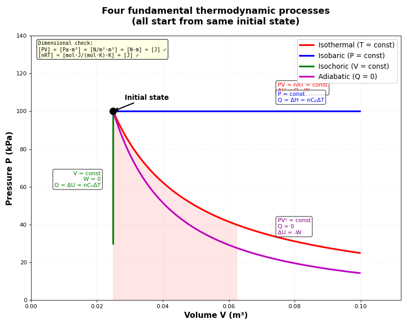
Four fundamental processes: (see Isothermal process (constant temperature), Isochoric process (constant volume), and Adiabatic process (no heat transfer))
Process |
Constraint |
Heat relation |
Work |
|---|---|---|---|
Isothermal |
\(\Delta T = 0\) |
\(Q = -W\) |
\(W = nRT\ln(V_1/V_2)\) |
Isobaric |
\(\Delta P = 0\) |
\(Q = \Delta H\) |
\(W = -P\Delta V\) |
Isochoric |
\(\Delta V = 0\) |
\(Q = \Delta U\) |
\(W = 0\) |
Adiabatic |
\(Q = 0\) |
\(Q = 0\) |
\(W = nC_V(T_2 - T_1)\) |
Key thermodynamic relations:
Relation |
Formula |
|---|---|
Heat capacity at constant P |
\(C_P = \left(\frac{\partial H}{\partial T}\right)_P\) |
Heat capacity at constant V |
\(C_V = \left(\frac{\partial U}{\partial T}\right)_V\) |
Heat capacity difference |
\(C_P - C_V = \frac{TV\alpha^2}{\kappa_T}\) |
Ideal gas |
\(C_P - C_V = nR\) |
Carnot efficiency |
\(\eta = 1 - \frac{T_C}{T_H}\) (see Heat engines and the Carnot cycle) |
Adiabatic process |
\(PV^{\gamma} = \text{const}, \quad TV^{\gamma-1} = \text{const}\) (see Adiabatic process (no heat transfer)) |
Clausius-Clapeyron |
\(\ln(P_2/P_1) = -\frac{\Delta H_{\text{vap}}}{R}\left(\frac{1}{T_2} - \frac{1}{T_1}\right)\) (see Clausius-Clapeyron equation) |
Material response coefficients: (see Second derivative relations)
Coefficient |
Definition |
|---|---|
Thermal expansion |
\(\alpha = \frac{1}{V}\left(\frac{\partial V}{\partial T}\right)_P\) |
Isothermal compressibility |
\(\kappa_T = -\frac{1}{V}\left(\frac{\partial V}{\partial P}\right)_T\) |
Part I: Fundamental Laws
Thermodynamics governs how energy flows and transforms in physical systems. Before diving into mathematical formalism, consider what thermodynamics explains: Why does heat flow from hot to cold? Why can’t we build a perpetual motion machine? Why do ice cubes melt in warm water but never spontaneously form? The answers lie in three fundamental laws that form the foundation of this theory.
First law of thermodynamics
- Why do we need the first law?
In the 18th and 19th centuries, scientists observed that mechanical work could generate heat (friction) and heat could produce mechanical work (steam engines). The first law formalizes a profound insight: energy is conserved - it can change forms (mechanical → thermal → chemical) but the total amount never changes.
This was not obvious historically. Early theories treated “heat” and “work” as fundamentally different phenomena. The first law unified them as different manifestations of energy transfer.
- What is the first law?
The first law of thermodynamics states that energy is conserved. The change in internal energy of a system equals the sum of heat transferred into the system and work done on the system.
Mathematically, for any process:
\[\Delta U = Q + W\]where \(\Delta U\) is the change in internal energy, \(Q\) is heat added to the system, and \(W\) is work done on the system.
- What is internal energy?
Internal energy \(U\) is the total energy contained within a system, including:
Kinetic energy of molecular motion (translational, rotational, vibrational)
Potential energy from intermolecular forces
Chemical bond energies
Electronic excitation energies
Crucially, \(U\) is a state function: it depends only on the current state (T, P, V, composition), not on how the system got there. This contrasts with heat \(Q\) and work \(W\), which are path-dependent.
- Why are heat and work path-dependent?
Consider taking a gas from state A (300 K, 1 atm) to state B (400 K, 2 atm). The change in internal energy \(\Delta U\) is the same regardless of path, but the amounts of heat and work depend on how we do it:
Path 1: Heat at constant volume, then compress isothermally
Path 2: Compress adiabatically (no heat), then heat at constant pressure
Path 3: Heat and compress simultaneously
Each path has the same \(\Delta U\) but different \(Q\) and \(W\). This is why we write \(dU\) (exact differential) but \(\delta Q\) and \(\delta W\) (inexact differentials).
General form of the first law:
The most general expression for the first law includes all possible types of work:
\[dU = \delta Q + \delta W + \delta W'\]where:
\(dU\) = incremental change in internal energy (state function)
\(\delta Q\) = heat transferred into or out of the system (path-dependent)
\(\delta W\) = mechanical work, typically pressure-volume work or stress-strain work (path-dependent)
\(\delta W'\) = other types of work (path-dependent), including:
Chemical work (changing composition)
Electrical work (moving charges in electric field)
Magnetic work (magnetization/demagnetization)
Surface work (changing surface area)
Simplified form for simple compressible systems:
For most thermodynamic problems involving simple systems without chemical, electrical, or magnetic effects:
\[dU = \delta Q + \delta W\]For a reversible process with only pressure-volume work:
\[dU = \delta Q - PdV\]where the negative sign reflects the sign convention (see below).
- What is the difference between work and heat?
Work and heat can both be measured in the same unit of energy, but they are fundamentally different in nature. On a microscopic level, heat is associated with the random motion of molecules, while work involves organized motion in a specific direction. For example, the random molecular motion in hot water represents heat transfer from the surroundings, whereas when the beaker slides across the desk due to friction, mechanical work is being done.
- What is the sign convention for work in materials science and engineering?
When the system does work on the surroundings (for example, expansion work), energy leaves the system, so the work is considered negative. This gives \(\delta W = -PdV\) for pressure-volume work.
Expansion (\(dV > 0\)): System does work on surroundings → \(\delta W < 0\) → Internal energy decreases
Compression (\(dV < 0\)): Surroundings do work on system → \(\delta W > 0\) → Internal energy increases
Note
Sign convention warning: Some physics textbooks use the opposite convention where work done by the system is positive. Always check the sign convention when comparing results across different sources.
- Can you observe (with your eyes) a reversible process?
No, a reversible process cannot be directly observed with the naked eye. For example, consider ice and water in equilibrium at 0 °C. Although nothing appears to change macroscopically, at the microscopic level there is a continuous, infinitesimal exchange of molecules between the solid and liquid phases—some water molecules freeze while others melt.
- What is required to have a reversible process?
A reversible process requires the system to remain infinitesimally close to equilibrium at every instant. This demands:
Infinitesimal gradients: Temperature, pressure, and chemical potential differences must be infinitesimal
Infinitely slow execution: The process must proceed quasi-statically
No dissipative effects: No friction, turbulence, or other irreversible mechanisms
In practice, reversible processes are idealizations. Real processes are always irreversible to some degree, but slow, carefully controlled processes can approximate reversibility.
- What is an isolated system?
An isolated system has no exchange of energy (neither heat nor work) and no exchange of matter with its surroundings. Hence, its total energy and mass are constant.
Examples:
The universe as a whole (by definition)
A perfectly insulated, rigid, sealed container (approximation)
- Why is the universe considered “isolated”?
We assume that the universe contains everything, so by definition there is nothing external with which to exchange heat, work, or matter. This makes the universe the ultimate isolated system, and the first law tells us that the total energy of the universe is constant.
Second law of thermodynamics
- Why do we need the second law?
The first law tells us energy is conserved, but it doesn’t explain directionality. Why does heat flow from hot to cold and never the reverse (without external work)? Why do gases expand into vacuum spontaneously? Why can’t we extract work from the ocean by cooling it slightly?
The first law alone would allow all these “forbidden” processes - they would conserve energy. We need the second law to explain why nature has a preferred direction: toward increasing disorder (entropy).
Historically, the second law emerged from studying heat engines. Engineers noticed that no engine could convert heat completely into work - some heat must always be rejected. This practical observation led to the profound concept of entropy.
- What does the second law state for isolated systems?
During spontaneous transformations, the entropy of an isolated system increases: \(dS_{\text{univ}} \geq 0\).
For reversible processes: \(dS_{\text{univ}} = 0\)
For irreversible processes: \(dS_{\text{univ}} > 0\)
Note: This can be derived but is given as a fundamental law (axiom).
Derivation: Show \(dS \geq \frac{(\delta Q)_{\text{irr}}}{T}\)
Key setup: Consider two different processes (one reversible, one irreversible) that take a system from the same initial state (state A) to the same final state (state B). For example, both processes might take a gas from \((P_1, V_1, T_1)\) to \((P_2, V_2, T_2)\).
Since internal energy \(U\) is a state function, its change depends only on the initial and final states, not on the path taken between them. Therefore:
Or in differential form:
From the first law, for both processes:
Since \(dU_{\text{rev}} = dU_{\text{irr}}\), we can equate these:
Rearranging:
We already know \((\delta W)_{\text{irr}} > (\delta W)_{\text{rev}}\) (shown below), which means \((\delta W)_{\text{rev}} - (\delta W)_{\text{irr}} < 0\).
Therefore:
For a reversible process, \(dS = \frac{(\delta Q)_{\text{rev}}}{T}\), so:
Therefore:
Derivation: Show \((\delta W)_{\text{irr}} > (\delta W)_{\text{rev}}\)
By definition, \(\delta W = -P_{\text{ext}}dV\).
For reversible process: \(\delta W_{\text{rev}} = -PdV\) where \(P \approx P_{\text{ext}}\) (equilibrium).
For irreversible process: \(\delta W_{\text{irr}} = -P_{\text{ext}}dV\) where \(P_{\text{ext}}\) differs from \(P\).
Compression (work done on system, \(dV < 0\)):
\(\delta W_{\text{irr}} = -(P_{\text{ext}} - P)dV\) where \(P_{\text{ext}} > P\)
Since \(dV < 0\): \(\delta W_{\text{irr}} > \delta W_{\text{rev}}\)
Expansion (work done by system, \(dV > 0\)):
\(\delta W_{\text{rev}} = -PdV\) (more negative, system does more work)
\(\delta W_{\text{irr}} = -P_{\text{ext}}dV\) where \(P_{\text{ext}} < P\)
Since \(dV > 0\) and \(P_{\text{ext}} < P\): \(\delta W_{\text{irr}} > \delta W_{\text{rev}}\)
Therefore: \(\delta W_{\text{irr}} \geq \delta W_{\text{rev}}\) (equality for reversible process).
Third law of thermodynamics
- What does the third law state?
The third law of thermodynamics states that the entropy of a perfect crystal approaches zero as the temperature approaches absolute zero:
\[\lim_{T \to 0} S = 0 \quad \text{(for a perfect crystal)}\]This provides an absolute reference point for entropy, unlike energy which only has relative values.
- Why is the third law important?
The third law has several profound implications:
1. Absolute entropy becomes calculable
Unlike internal energy (where we can only measure changes \(\Delta U\)), entropy has an absolute zero point. We can calculate the absolute entropy of any substance at temperature T:
\[S(T) = \int_0^T \frac{C_P(T')}{T'} dT'\]This integral starts from S = 0 at T = 0 and accumulates entropy as temperature increases.
2. Unattainability of absolute zero
The third law implies that it’s impossible to reach absolute zero in a finite number of steps. As \(T \to 0\), the heat capacity \(C_P \to 0\), making it progressively harder to extract energy and lower the temperature further.
3. Behavior of heat capacity at low temperatures
For the entropy to remain finite as \(T \to 0\), the heat capacity must vanish:
\[\lim_{T \to 0} C_P = 0\]Experimentally, heat capacities follow \(C_P \propto T^3\) (Debye model) at low temperatures, consistent with the third law.
4. Phase transitions at T = 0
The Clausius-Clapeyron equation \(\frac{dP}{dT} = \frac{\Delta S}{\Delta V}\) implies that phase transition lines in a P-T diagram must have zero slope as \(T \to 0\) (since \(\Delta S \to 0\)).
- What about imperfect crystals?
Real materials often have residual entropy at T = 0 due to disorder:
Molecular orientations: CO molecules in a crystal can point either way (C-O or O-C), giving \(S_0 = R \ln 2\) per mole
Spin glasses: Magnetic spins frozen in random configurations
Structural disorder: Defects, grain boundaries, mixed occupancy sites
The third law applies strictly only to perfect crystals in thermodynamic equilibrium. Glasses and amorphous materials can have significant residual entropy.
Connection to statistical mechanics
- What is the statistical interpretation of the third law?
Boltzmann’s entropy formula connects thermodynamics to statistical mechanics:
\[S = k_B \ln \Omega\]where \(k_B\) is Boltzmann’s constant and \(\Omega\) is the number of microscopic states (microstates) corresponding to a macroscopic state.
At T = 0, a perfect crystal has only one accessible microstate (the ground state), so:
\[S(T=0) = k_B \ln 1 = 0\]This provides a microscopic understanding: zero entropy means zero configurational uncertainty.
Reversible vs irreversible processes and entropy of the universe
- How does entropy change in reversible and irreversible processes?
There are really two ways the entropy of a system can change:
\[dS = \underbrace{\frac{\delta q_{\text{rev}}}{T}}_{\text{entropy transfer}} + \underbrace{dS_{\text{gen}}}_{\text{entropy production}}\]where
\(\frac{\delta q_{\text{rev}}}{T}\) is the entropy transferred to or from the system by heat exchange (if the same heat had been transferred reversibly at temperature \(T\)), and
\(dS_{\text{gen}} \geq 0\) is the entropy produced within the system by irreversibilities (like friction, viscous flow, diffusion, etc.).
- What happens in a reversible process?
Reversible process:
\[dS_{\text{gen}} = 0\]No entropy is produced internally because the system is in perfect equilibrium at every step.
Therefore, for the universe (system + surroundings):
\[\Delta S_{\text{univ}} = \Delta S_{\text{sys}} + \Delta S_{\text{surr}} = 0\]The universe’s entropy is conserved (no creation, no destruction).
Why is no entropy produced in a reversible process?
Rather than accepting \(dS_{\text{gen}} = 0\) as a rule, the deeper reason lies in examining what causes entropy production.
Entropy production requires finite gradients
Entropy is produced whenever a process involves finite gradients — a finite temperature difference, pressure difference, chemical potential difference, or any other driving force that pushes the system out of equilibrium. These gradients cause spontaneous flows of heat, matter, or momentum, and those flows are inherently irreversible.
Examples of finite gradients causing irreversibility:
Heat flow: If \(T_{\text{hot}} - T_{\text{cold}}\) is finite, heat flows spontaneously from hot to cold, producing entropy
Gas expansion: If \(P_{\text{inside}} - P_{\text{outside}}\) is finite, gas rushes out, producing entropy through turbulence and friction
Chemical reaction: If \(\mu_{\text{reactants}} - \mu_{\text{products}}\) is finite, the reaction proceeds spontaneously in one direction, producing entropy
Diffusion: If there is a finite concentration gradient, particles diffuse down the gradient, producing entropy
Reversible process = infinitesimal gradients
A truly reversible process proceeds through a series of equilibrium states where all gradients are infinitesimal:
Temperature difference: \(\Delta T \to 0\)
Pressure difference: \(\Delta P \to 0\)
Chemical potential difference: \(\Delta \mu \to 0\)
With infinitesimal gradients, the system remains in equilibrium at every instant. There are no spontaneous flows, no dissipation, and therefore no entropy production.
Formal relationship
For a reversible process, since \(T_{\text{sys}} = T_{\text{surr}}\) at every instant, the total entropy change is:
The entropy transferred out of the surroundings exactly equals the entropy transferred into the system, with no entropy created in the process.
Why reversible processes are idealized limits
The requirement for infinitesimal gradients means:
Processes must proceed infinitely slowly (quasi-static)
Any real process happening at finite speed must have finite gradients
Therefore, all real processes produce entropy and are irreversible
Key insight: Entropy production is the signature of finite gradients. No gradients = no spontaneous flows = no entropy production = reversible process.
- What happens in an irreversible process?
Irreversible process:
\[dS_{\text{gen}} > 0\]Entropy is produced inside the system or surroundings due to real world imperfections.
Therefore:
\[\Delta S_{\text{univ}} = \Delta S_{\text{sys}} + \Delta S_{\text{surr}} > 0\]The universe’s entropy increases.
- Why does this matter for the universe?
The second law tells us that the universe always moves in the direction of increasing entropy. Every real process (which is irreversible) creates entropy, making the universe’s total entropy grow.
Key insight: Reversible processes are idealized limits used for calculations, but they do not actually occur in nature. All real processes are irreversible and generate entropy, driving the universe toward higher entropy states.
Spontaneous processes that increase the universe’s entropy:
Heat flows from hot to cold
Gases expand into vacuum
Chemical reactions proceed in one direction
The reverse processes (such as heat flowing from cold to hot without work input) would decrease universe entropy and thus violate the second law.
- Can we reverse an irreversible process?
Yes, but it requires external work input. For example, a refrigerator transfers heat from cold to hot, but it requires electrical work to do so. The total entropy change of the universe (including the power plant generating the electricity) is still positive.
The key point: While we can decrease a system’s entropy locally, we always increase the universe’s total entropy in the process.
Conditions of equilibrium
- What does it mean for a system to be in equilibrium?
Equilibrium occurs when entropy is maximized for the given constraints. At equilibrium, the system has no tendency to change spontaneously. Any virtual (infinitesimal) transfer of energy, volume, or matter between subsystems produces no change in total entropy: \(dS = 0\).
- Why is temperature the same at equilibrium?
Temperature equality at equilibrium follows directly from entropy maximization. Consider two subsystems in thermal contact that can exchange energy.
Derivation of temperature equality:
Consider an isolated system composed of two subsystems (1 and 2) that can exchange energy but have fixed volumes and particle numbers. The total entropy is additive:
\[S = S^{(1)}(U^{(1)}, V^{(1)}, N_j^{(1)}) + S^{(2)}(U^{(2)}, V^{(2)}, N_j^{(2)})\]Since the overall system is isolated, total energy is conserved:
\[U^{(1)} + U^{(2)} = \text{constant}\]Therefore:
\[dU^{(1)} = -dU^{(2)}\]At equilibrium, entropy is maximized, so any virtual energy transfer must give \(dS = 0\):
\[dS = \left(\frac{\partial S^{(1)}}{\partial U^{(1)}}\right)_{V^{(1)}, N_j^{(1)}} dU^{(1)} + \left(\frac{\partial S^{(2)}}{\partial U^{(2)}}\right)_{V^{(2)}, N_j^{(2)}} dU^{(2)}\]From the intensive parameter definitions (see Intensive parameters from entropic representation):
\[\left(\frac{\partial S}{\partial U}\right)_{V,N} = \frac{1}{T}\]Substitute this and use \(dU^{(1)} = -dU^{(2)}\):
\[dS = \frac{1}{T^{(1)}} dU^{(1)} + \frac{1}{T^{(2)}} dU^{(2)} = \frac{1}{T^{(1)}} dU^{(1)} - \frac{1}{T^{(2)}} dU^{(1)}\]\[dS = \left(\frac{1}{T^{(1)}} - \frac{1}{T^{(2)}}\right) dU^{(1)}\]For equilibrium, this must vanish for arbitrary values of \(dU^{(1)}\):
\[\frac{1}{T^{(1)}} - \frac{1}{T^{(2)}} = 0\]Therefore:
\[T^{(1)} = T^{(2)}\]This shows that at thermal equilibrium, temperatures must be equal. If temperatures were different, entropy could increase by spontaneous energy transfer from hot to cold.
- What is the stability condition for equilibrium?
For true equilibrium, entropy must not just be an extremum (dS = 0) but a maximum. This requires the second derivative to be negative:
\[d^2S < 0\]This condition ensures the system is stable. If d²S were positive, the system would be at a minimum of entropy (unstable) and would spontaneously move away from that state. If d²S = 0, further analysis of higher derivatives would be needed.
Physical meaning of the stability condition:
The stability condition d²S < 0 means that any small fluctuation away from equilibrium will decrease entropy, so the system will spontaneously return to the equilibrium state. This ensures the equilibrium is stable rather than unstable or metastable.
For example, in thermal equilibrium:
If system 1 spontaneously gains a small amount of energy \(\delta U\), entropy must decrease: \(\delta^2 S < 0\)
This creates a restoring tendency that brings the system back to equal temperatures
The system is stable against small thermal fluctuations
Intensive parameters from entropic representation
- What are intensive parameters in thermodynamics?
Intensive parameters are properties that do not depend on system size (like temperature, pressure, chemical potential). They can be derived as partial derivatives of entropy with respect to extensive variables (energy, volume, particle number).
Entropic representation:
For a system with entropy \(S(U, V, N_1, ..., N_r)\) as a function of internal energy \(U\), volume \(V\), and particle numbers \(N_j\):
\[\left(\frac{\partial S}{\partial U}\right)_{V, N_1,...,N_r} = \frac{1}{T}\]\[\left(\frac{\partial S}{\partial V}\right)_{U, N_1,...,N_r} = \frac{P}{T}\]\[\left(\frac{\partial S}{\partial N_j}\right)_{U, V, N_{i \neq j}} = -\frac{\mu_j}{T}\]where \(\mu_j\) is the chemical potential of species \(j\).
Derivation from energetic representation:
These relations can be derived by inverting the energetic representation. Start with entropy as a state function:
\[S = S(U, V, N_1, ..., N_r)\]The differential is:
\[dS = \left(\frac{\partial S}{\partial U}\right)_{V,N} dU + \left(\frac{\partial S}{\partial V}\right)_{U,N} dV + \sum_j \left(\frac{\partial S}{\partial N_j}\right)_{U,V,N_{i \neq j}} dN_j\]From the first law with chemical work included:
\[dU = TdS - PdV + \sum_j \mu_j dN_j\]Rearrange to express \(dS\):
\[TdS = dU + PdV - \sum_j \mu_j dN_j\]\[dS = \frac{1}{T}dU + \frac{P}{T}dV - \sum_j \frac{\mu_j}{T} dN_j\]Comparing coefficients with the first expression:
\[\left(\frac{\partial S}{\partial U}\right)_{V,N} = \frac{1}{T}\]\[\left(\frac{\partial S}{\partial V}\right)_{U,N} = \frac{P}{T}\]\[\left(\frac{\partial S}{\partial N_j}\right)_{U,V,N_{i \neq j}} = -\frac{\mu_j}{T}\]Note the negative sign in the chemical potential term.
Combined first and second law:
Using these intensive parameters, we can write the fundamental relation:
\[dU = TdS - PdV + \mu_1 dN_1 + ... + \mu_r dN_r\]This combines the first law (energy conservation) with the second law (entropy definition) for an open system where particle numbers can change.
Compare with the statement of the first law:
\[dU = \delta Q + \delta W_M + \delta W_c\]where:
\(\delta Q = TdS\) for quasi-static heat flux
\(\delta W_M = -PdV\) is mechanical work
\(\delta W_c = \sum_j \mu_j dN_j\) is chemical work
All work terms (\(\delta W_M\) and \(\delta W_c\)) are process variables (path-dependent), while \(dU\) and \(dS\) are state functions.
Summary of Part I
Part I established the three fundamental laws:
The first law (energy conservation): \(dU = \delta Q - PdV\)
The second law (entropy increase): \(dS \geq \delta Q/T\)
The third law (absolute entropy): \(\lim_{T \to 0} S = 0\)
Equilibrium conditions from entropy maximization
Reversible vs irreversible processes and entropy production
The Unary systems section (Euler equation, Gibbs-Duhem) has been moved to Part III with the mathematical framework.
Part II: Processes and Applications
This part covers the four fundamental thermodynamic processes and their practical applications. We begin with heat capacities (essential for understanding all processes), then examine each process type (see Isothermal process (constant temperature), Isochoric process (constant volume), Adiabatic process (no heat transfer)), and conclude with the Carnot cycle (see Heat engines and the Carnot cycle).

Heat capacities
- Why do we need to understand heat capacities first?
Heat capacities (C_P and C_V) appear in the governing equations for nearly every thermodynamic process. Understanding them is essential before studying how systems behave under different constraints.
- What are heat capacities and how are they defined?
Heat capacity is the amount of heat required to raise the temperature of a system by one degree. The value depends on whether the process occurs at constant pressure (C_P) or constant volume (C_V).
Heat capacity at constant pressure (Cₚ)
- How is heat capacity at constant pressure defined?
Heat capacity at constant pressure measures how much heat is needed to raise temperature when pressure is held constant.
Definition:
By definition, heat capacity at constant pressure is:
\[C_P = \left(\frac{\partial H}{\partial T}\right)_P = \left(\frac{\delta Q}{dT}\right)_P\]Dimensional check: [CP] = [J/(mol·K)] or [J/K] depending on whether it’s molar or total. Since [H] = [J/mol] and [T] = [K], we have [∂H/∂T] = [J/mol]/[K] = [J/(mol·K)] ✓
The equality \(C_P = \left(\frac{\partial H}{\partial T}\right)_P\) follows from the fact that \(\delta Q = dH\) at constant pressure (see Why does heat equal enthalpy change at constant pressure?), so measuring heat flux at fixed pressure directly measures how enthalpy changes with temperature.
This is the differential (infinitesimal) form. For a small change in temperature \(dT\):
\[\delta Q = C_P dT\]
Integration for finite temperature changes:
For finite changes from \(T_1\) to \(T_2\), integrate both sides:
\[Q = \int_{T_1}^{T_2} \delta Q = \int_{T_1}^{T_2} C_P dT\]Since \(Q = \Delta H\) at constant pressure (see Why does heat equal enthalpy change at constant pressure?):
\[Q = \Delta H = \int_{T_1}^{T_2} C_P dT\]If \(C_P\) is constant (or approximately constant) over the temperature range, this simplifies to:
\[Q = \Delta H = C_P \Delta T = C_P(T_2 - T_1)\]
Example 2.1: Heating water and measuring C_P experimentally
Problem: You heat 500 g of water from 20°C to 80°C in a constant-pressure calorimeter. The heat supplied is 125,400 J. Calculate C_P for water and compare to the literature value.
Solution:
Using the relation Q = C_P ΔT at constant pressure:
In molar units (M_H₂O = 18 g/mol):
Comparison: The literature value is 75.3 J/(mol·K), so our measurement is within 0.1%!
Practical measurement technique:
Calorimeter setup: Insulated container to minimize heat loss
Electric heater: Known power P (watts) run for time t gives Q = Pt
Temperature measurement: Precise thermometer or thermocouple
Corrections: Account for heat capacity of container and heat losses
Why constant pressure? Open container at atmospheric pressure ensures P = constant, so the measured heat directly gives ΔH = Q.
Example 2.2: Enthalpy change for non-constant C_P
Problem: For many solids, C_P varies with temperature as C_P(T) = a + bT + c/T². For copper, a = 22.64 J/(mol·K), b = 6.28×10⁻³ J/(mol·K²), c = 0. Calculate ΔH when heating 1 mole of copper from 298 K to 1000 K.
Solution:
Use the integral form:
Key insight: If we incorrectly assumed C_P constant at the average value C_P(649 K) ≈ 26.7 J/(mol·K), we would get:
The error is only 0.06% because the temperature dependence is weak for this range. But for larger ΔT or stronger temperature dependence, integration is essential!
Heat capacity at constant volume (Cᵥ)
- How is heat capacity at constant volume defined?
Heat capacity at constant volume measures how much heat is needed to raise temperature when volume is held constant. From the first law for a reversible process:
\[dU = \delta Q_{\text{rev}} - PdV\]For a reversible process, \(\delta Q_{\text{rev}} = TdS\) (from the second law), so:
\[dU = TdS - PdV\]This expression tells us how \(U\) changes with \(S\) and \(V\):
\[\left(\frac{\partial U}{\partial S}\right)_V = T\]\[\left(\frac{\partial U}{\partial V}\right)_S = -P\]Natural variables for \(U\) are \((S, V)\) (entropy and volume).
Special thermodynamic processes
With heat capacities defined, we now examine the four fundamental processes. Each process imposes a different constraint (constant T, P, V, or Q=0), leading to different simplified forms of the first law.
Isothermal process (constant temperature)
- What happens in an isothermal process?
An isothermal process occurs at constant temperature. For an ideal gas, this means the internal energy remains constant (\(\Delta U = 0\)), so all heat absorbed is converted to work (or vice versa).
Starting from the first law:
\[dU = \delta Q - PdV\]For an ideal gas at constant temperature, \(dU = 0\), so:
\[\delta Q = PdV\]This means heat input equals work output (or heat removal equals work input).
Work done in isothermal expansion/compression:
For an ideal gas \(PV = nRT\), we have \(P = nRT/V\). The work is:
\[W = -\int_{V_1}^{V_2} P dV = -\int_{V_1}^{V_2} \frac{nRT}{V} dV = -nRT \ln\frac{V_2}{V_1}\]For expansion (\(V_2 > V_1\)), \(W < 0\) (system does work on surroundings). For compression (\(V_2 < V_1\)), \(W > 0\) (work done on system).
Heat transfer:
Since \(\Delta U = 0\):
\[Q = -W = nRT \ln\frac{V_2}{V_1}\]
Example 2.3: Isothermal expansion of an ideal gas
Problem: One mole of an ideal gas at 300 K expands isothermally from 10 L to 20 L. Calculate:
The work done by the gas
The heat absorbed
The change in internal energy
Solution:
Given: n = 1 mol, T = 300 K, V₁ = 10 L, V₂ = 20 L, R = 8.314 J/(mol·K)
Part 1: Work done
The negative sign means work is done BY the gas (expansion).
Note
Dimensional analysis: The work formula \(W = -nRT \ln(V_2/V_1)\) has correct energy units:
\([nRT] = \text{mol} \times \frac{\text{J}}{\text{mol·K}} \times \text{K} = \text{J}\) ✓
\(\ln(V_2/V_1)\) is dimensionless (ratio of volumes) ✓
Therefore \([W] = \text{J}\) (energy) ✓
Part 2: Heat absorbed
For an isothermal process of an ideal gas, \(Q = -W\):
The gas absorbs 1729 J of heat from the surroundings.
Part 3: Internal energy change
For an ideal gas at constant temperature:
Energy accounting:
Heat in: +1729 J
Work out: -1729 J
Net change in U: 0 J ✓
Physical interpretation: At constant temperature, all the absorbed heat is converted into work to push against external pressure during expansion. The temperature stays constant because heat flows in at exactly the rate needed to compensate for the cooling effect of expansion.
Isochoric process (constant volume)
- What happens in an isochoric process?
For a process at constant volume \(V\), no pressure-volume work is done, and heat directly changes internal energy.
Starting from the first law:
\[dU = \delta Q - PdV\]At constant volume, \(dV = 0\):
\[\delta Q = dU \quad \text{(at constant volume)}\]Therefore, all heat transferred goes into changing internal energy.
No pressure-volume work:
\[W = -\int PdV = 0 \quad \text{(since } dV = 0 \text{)}\]
Adiabatic process (no heat transfer)
- What happens in an adiabatic process?
An adiabatic process occurs when a system undergoes a change without exchanging heat with its surroundings. This means \(\delta Q = 0\). Adiabatic conditions arise when:
The system is thermally insulated
The process happens so rapidly that there is no time for heat transfer
The system is perfectly isolated
In adiabatic processes, all energy change comes from work, so compression heats the gas while expansion cools it.
Starting from the first law:
\[dU = \delta Q - PdV\]For an adiabatic process, \(\delta Q = 0\):
\[dU = -PdV\]This means all internal energy change comes from work. For an ideal gas, \(dU = nC_V dT\), so:
\[nC_V dT = -PdV\]
Deriving the PV relationship:
For an ideal gas \(PV = nRT\), we can write \(P = nRT/V\). Substituting:
\[nC_V dT = -\frac{nRT}{V}dV\]Dividing both sides by \(nT\):
\[\frac{C_V dT}{T} = -\frac{R dV}{V}\]Integrate both sides:
\[C_V \ln T = -R \ln V + \text{const}\]Rearranging using \(\gamma = C_P/C_V\) and \(C_P - C_V = R\) (which gives \(R = C_V(\gamma - 1)\)):
\[TV^{\gamma-1} = \text{constant}\]We can also eliminate \(T\) using \(PV = nRT\) to obtain:
\[PV^{\gamma} = \text{constant}\]These are the fundamental relationships for adiabatic processes of an ideal gas.
Work done in an adiabatic process:
The work done can be calculated from \(dU = -PdV\):
\[W = -\int_{V_1}^{V_2} P dV\]Using \(PV^{\gamma} = P_1V_1^{\gamma}\), we get \(P = P_1V_1^{\gamma}/V^{\gamma}\):
\[W = -P_1V_1^{\gamma} \int_{V_1}^{V_2} V^{-\gamma} dV = -P_1V_1^{\gamma} \left[\frac{V^{1-\gamma}}{1-\gamma}\right]_{V_1}^{V_2}\]Simplifying:
\[W = \frac{P_1V_1^{\gamma}}{(\gamma-1)} \left(V_2^{1-\gamma} - V_1^{1-\gamma}\right) = \frac{P_2V_2 - P_1V_1}{\gamma-1}\]Since \(PV = nRT\):
\[W = \frac{nR(T_2 - T_1)}{\gamma-1} = nC_V(T_2 - T_1)\]For adiabatic compression (\(V_2 < V_1\)), \(T_2 > T_1\) (temperature increases) and \(W > 0\) (work done on the gas). For adiabatic expansion (\(V_2 > V_1\)), \(T_2 < T_1\) (temperature decreases) and \(W < 0\) (gas does work on surroundings).
Example 2.4: Adiabatic compression in a diesel engine
Problem: A diesel engine compresses air (γ = 1.4) from 1.00 L to 0.050 L. Initial conditions are T₁ = 300 K and P₁ = 1.0 atm. Calculate the final temperature and pressure.
Solution:
Using the adiabatic relation \(TV^{\gamma-1} = \text{constant}\):
For pressure, using \(PV^{\gamma} = \text{constant}\):
Physical interpretation: The compression ratio of 20:1 produces temperatures high enough to spontaneously ignite diesel fuel without a spark plug. This is how diesel engines work!
Comparison table of the four processes
Summary of the four fundamental processes:
Process type
First law simplifies
Heat relation
Work
Isothermal
\(\Delta U = 0\)
\(Q = -W\)
\(W = nRT\ln(V_1/V_2)\)
Isobaric
\(Q = \Delta H\)
\(Q = C_P\Delta T\)
\(W = -P\Delta V\)
Isochoric
\(Q = \Delta U\)
\(Q = C_V\Delta T\)
\(W = 0\)
Adiabatic
\(\Delta U = W\)
\(Q = 0\)
\(W = nC_V(T_2 - T_1)\)
Note how heat capacities C_P and C_V appear in three of the four processes - this is why we studied them first!
Summary of Part II
Part II established the practical foundations of thermodynamics:
Heat capacities (C_P and C_V) quantify how materials respond to heating at different constraints
Four fundamental processes: isothermal, isobaric, isochoric, and adiabatic
Comparison table summarizing work and heat relations for each process type
These tools enable quantitative calculations for real systems. Part II concludes with the premier application of the Second Law: the Carnot cycle.
Heat engines and the Carnot cycle

- What is the Carnot cycle and why is it important?
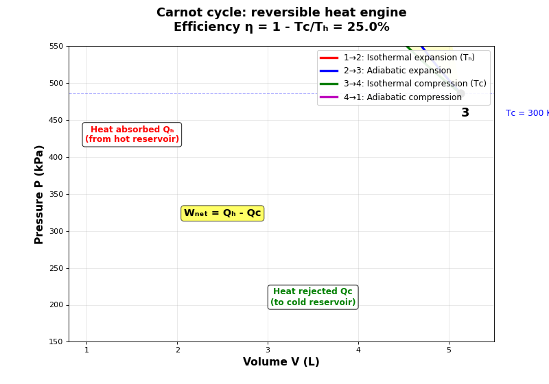
The Carnot cycle is a theoretical thermodynamic cycle that represents the most efficient possible heat engine operating between two temperatures. It consists of four reversible steps: two isothermal (see Isothermal process (constant temperature)) and two adiabatic processes (see Adiabatic process (no heat transfer)). The Carnot cycle is fundamental because:
It establishes the maximum possible efficiency for any heat engine
It demonstrates that entropy increases in the surroundings for any real (irreversible) engine
It provides a concrete connection between the Second Law and practical applications
Real engines (car engines, power plants) are limited by Carnot efficiency
The four steps of the Carnot cycle
- How does the Carnot cycle work?
A Carnot engine operates between a hot reservoir at temperature \(T_H\) and a cold reservoir at temperature \(T_C\). The working substance (typically an ideal gas) undergoes four reversible steps:
Step 1: Isothermal expansion at \(T_H\) (absorb heat)
The gas expands isothermally at \(T_H\), absorbing heat \(Q_H\) from the hot reservoir. Since the process is isothermal:
\(\Delta U_1 = 0\) (no change in internal energy for ideal gas at constant T)
Work done by gas: \(W_1 = nRT_H \ln\frac{V_2}{V_1}\)
Heat absorbed: \(Q_H = W_1 = nRT_H \ln\frac{V_2}{V_1}\)
Step 2: Adiabatic expansion \(T_H \to T_C\) (cool down)
The gas continues to expand adiabatically, doing work on the surroundings. No heat is transferred (\(Q_2 = 0\)). Temperature drops from \(T_H\) to \(T_C\):
Using the adiabatic relation (see Adiabatic process (no heat transfer)): \(T_H V_2^{\gamma-1} = T_C V_3^{\gamma-1}\)
Work done by gas: \(W_2 = nC_V(T_H - T_C)\)
Step 3: Isothermal compression at \(T_C\) (reject heat)
The gas is compressed isothermally at \(T_C\), rejecting heat \(Q_C\) to the cold reservoir:
\(\Delta U_3 = 0\)
Work done on gas: \(W_3 = nRT_C \ln\frac{V_4}{V_3}\) (negative since compression)
Heat rejected: \(Q_C = -W_3 = nRT_C \ln\frac{V_3}{V_4}\)
Step 4: Adiabatic compression \(T_C \to T_H\) (heat back up)
The gas is compressed adiabatically back to the initial state. Temperature rises from \(T_C\) to \(T_H\):
No heat transfer: \(Q_4 = 0\)
Adiabatic relation: \(T_C V_4^{\gamma-1} = T_H V_1^{\gamma-1}\)
Work done on gas: \(W_4 = nC_V(T_H - T_C)\) (positive, since compression increases temperature)
Carnot efficiency
- What is the efficiency of the Carnot cycle?
The efficiency η of a heat engine is defined as the ratio of net work output to heat input:
\[\eta = \frac{W_{\text{net}}}{Q_H} = \frac{Q_H - Q_C}{Q_H} = 1 - \frac{Q_C}{Q_H}\]
For the Carnot cycle:
From the isothermal steps:
Heat absorbed: \(Q_H = nRT_H \ln\frac{V_2}{V_1}\)
Heat rejected: \(Q_C = nRT_C \ln\frac{V_3}{V_4}\)
From the adiabatic steps (Steps 2 and 4):
\[T_H V_2^{\gamma-1} = T_C V_3^{\gamma-1}\]\[T_H V_1^{\gamma-1} = T_C V_4^{\gamma-1}\]Dividing these equations:
\[\frac{V_2^{\gamma-1}}{V_1^{\gamma-1}} = \frac{V_3^{\gamma-1}}{V_4^{\gamma-1}}\]Therefore: \(\frac{V_2}{V_1} = \frac{V_3}{V_4}\), which means \(\ln\frac{V_2}{V_1} = \ln\frac{V_3}{V_4}\).
The efficiency becomes:
\[\eta_{\text{Carnot}} = 1 - \frac{Q_C}{Q_H} = 1 - \frac{nRT_C \ln(V_3/V_4)}{nRT_H \ln(V_2/V_1)} = 1 - \frac{T_C}{T_H}\]The Carnot efficiency depends only on the temperatures of the two reservoirs:
\[\eta_{\text{Carnot}} = 1 - \frac{T_C}{T_H}\]This is the maximum possible efficiency for any heat engine operating between these two temperatures.
Note
Dimensional analysis: The Carnot efficiency \(\eta = 1 - T_C/T_H\) is dimensionless:
\([T_C/T_H] = \text{K}/\text{K}\) = dimensionless ✓
\([1 - T_C/T_H]\) = dimensionless ✓
Efficiency is a pure number (often expressed as percentage) ✓
Example: \(T_C = 300\text{ K}, T_H = 600\text{ K} \Rightarrow \eta = 1 - 300/600 = 0.5 = 50\%\)
Example 2.5: Power plant Carnot efficiency
Problem: A coal-fired power plant operates with steam at T_H = 540°C (813 K) and cooling water at T_C = 30°C (303 K). Calculate:
The maximum possible (Carnot) efficiency
If the plant absorbs Q_H = 1000 MW of heat, what is the maximum work output?
How much heat must be rejected to the cooling water?
Solution:
Part 1: Carnot efficiency
Part 2: Maximum work output
Part 3: Rejected heat
From energy conservation:
Reality check: Real coal plants achieve η ≈ 33-40%, roughly half the Carnot limit. This means:
Actual work output: ~350 MW (not 627 MW)
Actual rejected heat: ~650 MW (not 373 MW)
More cooling water needed and more thermal pollution
Why can’t we reach Carnot efficiency? Irreversibilities include:
Combustion (highly irreversible, finite ΔT)
Heat transfer through boiler tubes (finite ΔT)
Turbine friction and blade losses
Condenser inefficiencies
Example 2.6: Entropy production in a real engine
Problem: A real engine operates between T_H = 600 K and T_C = 300 K with efficiency η = 30% (compared to Carnot η_Carnot = 50%). If the engine absorbs Q_H = 100 kJ, calculate the total entropy change of the universe.
Solution:
Work and heat for the real engine:
Entropy changes:
Hot reservoir loses heat:
Cold reservoir gains heat:
Total entropy change of universe:
For comparison, a Carnot engine at the same Q_H:
For Carnot: Q_C = 50 kJ (from η = 50%), so:
Physical interpretation:
Real engine: Creates 66.6 J/K of entropy (irreversible)
Carnot engine: Creates 0 J/K of entropy (reversible limit)
Entropy production rate measures how far from ideal the real engine operates
This entropy production represents lost work potential that can never be recovered
Connection to the Second Law and entropy
- How does the Carnot cycle illustrate entropy?
The Carnot cycle demonstrates that even the most efficient possible engine produces entropy in the universe:
For the Carnot cycle (reversible):
Entropy change of working substance: \(\Delta S_{\text{gas}} = 0\) (returns to initial state)
Entropy change of hot reservoir: \(\Delta S_H = -\frac{Q_H}{T_H}\) (loses heat)
Entropy change of cold reservoir: \(\Delta S_C = +\frac{Q_C}{T_C}\) (gains heat)
Total entropy change of universe:
\[\Delta S_{\text{universe}} = \Delta S_H + \Delta S_C = -\frac{Q_H}{T_H} + \frac{Q_C}{T_C}\]For the reversible Carnot cycle, using \(Q_C = Q_H \frac{T_C}{T_H}\):
\[\Delta S_{\text{universe}} = -\frac{Q_H}{T_H} + \frac{Q_H T_C/T_H}{T_C} = -\frac{Q_H}{T_H} + \frac{Q_H}{T_H} = 0\]For a reversible Carnot engine, the total entropy of the universe remains constant. This is consistent with the Second Law: \(\Delta S_{\text{universe}} \geq 0\), with equality for reversible processes.
For any real (irreversible) engine:
Any real engine has efficiency \(\eta < \eta_{\text{Carnot}}\), meaning:
\[Q_C > Q_H \frac{T_C}{T_H}\]Therefore:
\[\Delta S_{\text{universe}} = -\frac{Q_H}{T_H} + \frac{Q_C}{T_C} > 0\]All real heat engines increase the entropy of the universe. The Carnot efficiency represents the limiting case where entropy increase is minimized to zero.
Real engines vs Carnot limit
- How do real engines compare to the Carnot limit?
No real engine can achieve Carnot efficiency because:
Friction and dissipation make processes irreversible
Finite temperature gradients are required for heat transfer (see discussion in reversible-vs-irreversible)
Finite time constraints prevent truly reversible operation
Example efficiencies:
Carnot limit (T_H = 600 K, T_C = 300 K): η_Carnot = 1 - 300/600 = 50%
Modern car engines: η ≈ 25-30%
Coal power plants: η ≈ 33-40%
Combined cycle gas turbines: η ≈ 50-60% (approaching Carnot limit with high T_H)
The Carnot cycle thus provides both a theoretical limit and a practical benchmark. Improving real engine efficiency means reducing irreversibilities to approach the Carnot limit.
Part III: Mathematical Framework
This part presents the mathematical machinery of thermodynamics: the four thermodynamic potentials (see Internal energy and its partial derivatives and Helmholtz free energy and its partial derivatives), Maxwell relations (see Maxwell relations), TdS equations (see TdS equations), and material properties (see Second derivative relations). These tools transform thermodynamics from qualitative principles into quantitative predictions.
Thermodynamic potentials
- What are thermodynamic potentials?
Thermodynamic potentials are state functions that characterize the equilibrium state of a system. Each potential is naturally suited for specific experimental conditions (which variables are held constant). The four main potentials are:
Internal energy \(U(S,V)\): Natural variables are entropy and volume (see Internal energy and its partial derivatives)
Enthalpy \(H(S,P)\): Natural variables are entropy and pressure (see Why does heat equal enthalpy change at constant pressure?)
Helmholtz free energy \(F(T,V)\): Natural variables are temperature and volume (see Helmholtz free energy and its partial derivatives)
Gibbs free energy \(G(T,P)\): Natural variables are temperature and pressure (see Gibbs free energy and volume)
These potentials form the foundation for deriving Maxwell relations and understanding phase equilibria.
Internal energy and its partial derivatives
- How does internal energy change with entropy and volume?
Internal energy \(U\) is a fundamental thermodynamic potential. The key relations are:
\[\left(\frac{\partial U}{\partial S}\right)_V = T\]\[\left(\frac{\partial U}{\partial V}\right)_S = -P\]These can be derived from the first law.
Derivation:
Gibbs free energy and volume
- How does Gibbs free energy change with pressure at constant temperature?
The key relation is:
\[\left(\frac{\partial G}{\partial P}\right)_T = V\]This can be derived from first principles.
Step 1: Start from the definition of Gibbs free energy
\[G = H - TS\]Take the differential:
\[dG = dH - TdS - SdT\]
Step 2: Replace dH using the first law
From the definition of enthalpy \(H = U + PV\):
\[dH = dU + PdV + VdP\]For a simple compressible system, \(dU = TdS - PdV\).
Substitute that into the previous equation:
\[dH = (TdS - PdV) + PdV + VdP = TdS + VdP\]
Step 3: Substitute dH back into dG
\[dG = (TdS + VdP) - TdS - SdT\]Simplify:
\[dG = VdP - SdT\]
Step 4: Identify the partial derivatives
This expression tells us how \(G\) changes with \(P\) and \(T\):
\[\left(\frac{\partial G}{\partial P}\right)_T = V\]\[\left(\frac{\partial G}{\partial T}\right)_P = -S\]Note
Dimensional analysis: Check that the Gibbs free energy relations have correct units:
\([(\partial G/\partial P)_T] = \text{J}/\text{Pa} = \text{J·m}^3/\text{J} = \text{m}^3 = [V]\) ✓
\([(\partial G/\partial T)_P] = \text{J}/\text{K} = [S]\) ✓
Therefore \(dG = VdP - SdT\) has units: \([\text{m}^3 \cdot \text{Pa}] - [\text{J/K} \cdot \text{K}] = \text{J} - \text{J} = \text{J}\) ✓
These relations are particularly useful for studying phase equilibria. See Clausius-Clapeyron equation for an application to phase transitions.
Helmholtz free energy and its partial derivatives
- How does Helmholtz free energy change with volume and temperature?
Helmholtz free energy \(F\) is the natural thermodynamic potential for systems at constant temperature and volume. The key relations are:
\[\left(\frac{\partial F}{\partial V}\right)_T = -P\]\[\left(\frac{\partial F}{\partial T}\right)_V = -S\]These can be derived from first principles.
Step 1: Start from the definition of Helmholtz free energy
\[F = U - TS\]Take the differential:
\[dF = dU - TdS - SdT\]
Step 2: Replace dU using the first law
For a simple compressible system, the first law gives:
\[dU = TdS - PdV\]Substitute that into the previous equation:
\[dF = (TdS - PdV) - TdS - SdT\]Simplify:
\[dF = -PdV - SdT\]
Step 3: Identify the partial derivatives
This expression tells us how \(F\) changes with \(V\) and \(T\):
\[\left(\frac{\partial F}{\partial V}\right)_T = -P\]\[\left(\frac{\partial F}{\partial T}\right)_V = -S\]These relations are fundamental for deriving Maxwell relations (see Maxwell relations).
Comparison with all four potentials:
Internal energy \((U)\): Natural variables are \((S, V)\) → \(dU = TdS - PdV\)
Enthalpy \((H)\): Natural variables are \((S, P)\) → \(dH = TdS + VdP\)
Helmholtz \((F)\): Natural variables are \((T, V)\) → \(dF = -SdT - PdV\)
Gibbs \((G)\): Natural variables are \((T, P)\) → \(dG = -SdT + VdP\)
Maxwell relations
- What are Maxwell relations and how are they derived?
Maxwell relations are equalities between partial derivatives that follow from the exactness of thermodynamic state functions. They connect seemingly unrelated thermodynamic quantities.
Note
Why Maxwell relations are powerful: They allow us to measure difficult-to-access quantities (like entropy changes) by measuring easily accessible ones (like pressure and temperature). For example, \(\left(\frac{\partial S}{\partial V}\right)_T = \left(\frac{\partial P}{\partial T}\right)_V\) lets us find how entropy changes with volume by simply measuring how pressure changes with temperature.
Example derivation: Show \(\left(\frac{\partial S}{\partial V}\right)_T = \left(\frac{\partial P}{\partial T}\right)_V\)
Start with Helmholtz free energy: \(F = F(T, V)\) (see Helmholtz free energy and its partial derivatives for the derivation of this expression).
The differential is:
\[dF = -SdT - PdV\]This means:
\[\left(\frac{\partial F}{\partial T}\right)_V = -S\]\[\left(\frac{\partial F}{\partial V}\right)_T = -P\]Since \(F\) is a state function, its second derivatives are independent of the order:
\[\frac{\partial^2 F}{\partial T \partial V} = \frac{\partial^2 F}{\partial V \partial T}\]Taking derivatives:
\[\frac{\partial}{\partial V}\left(\frac{\partial F}{\partial T}\right)_V = \frac{\partial}{\partial T}\left(\frac{\partial F}{\partial V}\right)_T\]\[\frac{\partial(-S)}{\partial V} = \frac{\partial(-P)}{\partial T}\]Therefore:
\[\left(\frac{\partial S}{\partial V}\right)_T = \left(\frac{\partial P}{\partial T}\right)_V\]This is one of the Maxwell relations derived from Helmholtz free energy.
Derivation from internal energy U(S,V):
Start with internal energy: \(U = U(S, V)\) (see Internal energy and its partial derivatives for the derivation of this expression).
The differential is:
This means:
Since \(U\) is a state function, its second derivatives are independent of order:
Taking derivatives:
Therefore:
Derivation from enthalpy H(S,P):
Start with enthalpy: \(H = H(S, P)\) (see Why does heat equal enthalpy change at constant pressure? for the derivation of this expression).
The differential is:
\[dH = TdS + VdP\]This means:
\[\left(\frac{\partial H}{\partial S}\right)_P = T\]\[\left(\frac{\partial H}{\partial P}\right)_S = V\]Since \(H\) is a state function:
\[\frac{\partial^2 H}{\partial S \partial P} = \frac{\partial^2 H}{\partial P \partial S}\]Taking derivatives:
\[\frac{\partial}{\partial P}\left(\frac{\partial H}{\partial S}\right)_P = \frac{\partial}{\partial S}\left(\frac{\partial H}{\partial P}\right)_S\]\[\frac{\partial(T)}{\partial P} = \frac{\partial(V)}{\partial S}\]Therefore:
\[\left(\frac{\partial T}{\partial P}\right)_S = \left(\frac{\partial V}{\partial S}\right)_P\]
Derivation from Gibbs free energy G(T,P):
Start with Gibbs free energy: \(G = G(T, P)\) (see Gibbs free energy and volume for the derivation of this expression).
The differential is:
\[dG = -SdT + VdP\]This means:
\[\left(\frac{\partial G}{\partial T}\right)_P = -S\]\[\left(\frac{\partial G}{\partial P}\right)_T = V\]Since \(G\) is a state function:
\[\frac{\partial^2 G}{\partial T \partial P} = \frac{\partial^2 G}{\partial P \partial T}\]Taking derivatives:
\[\frac{\partial}{\partial P}\left(\frac{\partial G}{\partial T}\right)_P = \frac{\partial}{\partial T}\left(\frac{\partial G}{\partial P}\right)_T\]\[\frac{\partial(-S)}{\partial P} = \frac{\partial(V)}{\partial T}\]Therefore:
\[\left(\frac{\partial S}{\partial P}\right)_T = -\left(\frac{\partial V}{\partial T}\right)_P\]
Summary of all four Maxwell relations:
From thermodynamic potential
Maxwell relation
\(U(S,V): dU = TdS - PdV\)
\(\left(\frac{\partial T}{\partial V}\right)_S = -\left(\frac{\partial P}{\partial S}\right)_V\)
\(H(S,P): dH = TdS + VdP\)
\(\left(\frac{\partial T}{\partial P}\right)_S = \left(\frac{\partial V}{\partial S}\right)_P\)
\(F(T,V): dF = -SdT - PdV\)
\(\left(\frac{\partial S}{\partial V}\right)_T = \left(\frac{\partial P}{\partial T}\right)_V\)
\(G(T,P): dG = -SdT + VdP\)
\(\left(\frac{\partial S}{\partial P}\right)_T = -\left(\frac{\partial V}{\partial T}\right)_P\)
These four relations are powerful tools for deriving relationships between measurable quantities. They arise purely from the mathematical structure of thermodynamic potentials.
TdS equations
- What are the TdS equations?
The TdS equations express entropy changes in terms of measurable quantities (temperature, volume, pressure). There are two particularly useful forms derived using Maxwell relations (see Maxwell relations).
Summary of TdS equations:
First TdS equation (T,V variables):
\[TdS = C_V dT + T\left(\frac{\partial P}{\partial T}\right)_V dV = C_V dT + \frac{\alpha T}{\kappa_T} dV\]Second TdS equation (T,P variables):
\[TdS = C_P dT - T\left(\frac{\partial V}{\partial T}\right)_P dP = C_P dT - \alpha T V dP\]
Derivation of first TdS equation (T,V variables)
Start with entropy as a function of temperature and volume: \(S = S(T, V)\).
The differential is:
From the definition of heat capacity at constant volume: \(C_V = T\left(\frac{\partial S}{\partial T}\right)_V\), so:
From the Maxwell relation (see Maxwell relations):
Substitute both into the differential:
Multiply through by T:
Using the relation \(\left(\frac{\partial P}{\partial T}\right)_V = \frac{\alpha}{\kappa_T}\) (derived from the definitions of α and κ_T via the triple product rule):
Derivation of second TdS equation (T,P variables)
Start with entropy as a function of temperature and pressure: \(S = S(T, P)\).
The differential is:
From the definition of heat capacity at constant pressure: \(C_P = T\left(\frac{\partial S}{\partial T}\right)_P\), so:
From the Maxwell relation (see Maxwell relations):
Substitute both into the differential:
Multiply through by T:
Using the definition of thermal expansion coefficient \(\alpha = \frac{1}{V}\left(\frac{\partial V}{\partial T}\right)_P\):
Applications:
These equations connect the abstract concept of entropy to measurable quantities like heat capacities and material properties (α, κ_T):
First TdS equation uses (T,V) as independent variables, useful when volume is controlled or known
Second TdS equation uses (T,P) as independent variables, useful for constant pressure processes (most common experimentally)
Both allow calculating entropy changes in real processes where temperature and volume (or pressure) change simultaneously
Thermodynamic potentials with (T,P) as independent variables
- How do we express thermodynamic potentials and volume with (T,P) as independent variables?
When temperature and pressure are the independent variables (most common experimental setup), we can express differentials of all thermodynamic quantities in terms of dT and dP. This leads to a unified framework using measurable properties.
Differential of volume V(T,P):
Volume as a function of temperature and pressure:
\[dV = \left(\frac{\partial V}{\partial T}\right)_P dT + \left(\frac{\partial V}{\partial P}\right)_T dP\]Using the definitions of α and κ_T:
\[dV = V\alpha dT - V\kappa_T dP\]
Complete table of differentials in (T,P) variables:
Thermodynamic potential
Differential in (T,P) variables
Entropy: \(S(T,P)\)
\(dS = \frac{C_P}{T}dT - V\alpha dP\)
Internal energy: \(U(T,P)\)
\(dU = (C_P - PV\alpha)dT + V(P\kappa_T - T\alpha)dP\)
Volume: \(V(T,P)\)
\(dV = V\alpha dT - V\kappa_T dP\)
Enthalpy: \(H(T,P)\)
\(dH = C_P dT + V(1 - T\alpha)dP\)
Helmholtz: \(F(T,P)\)
\(dF = -(S + PV\alpha)dT + PV\kappa_T dP\)
Gibbs: \(G(T,P)\)
\(dG = -SdT + VdP\)
Derivation of dU in (T,P) variables
Start with the fundamental relation and substitute TdS:
Substitute the TdS equation: \(TdS = C_P dT - \alpha TV dP\):
Substitute dV: \(dV = V\alpha dT - V\kappa_T dP\):
Collect terms:
Derivation of dH in (T,P) variables
Start with the fundamental relation for enthalpy:
Substitute the TdS equation: \(TdS = C_P dT - \alpha TV dP\):
Physical interpretation:
These expressions show how each thermodynamic potential responds to changes in temperature and pressure:
Gibbs free energy has the simplest form because (T,P) are its natural variables
Internal energy has a complex form because its natural variables are (S,V), not (T,P)
All expressions involve measurable quantities: C_P, α, κ_T, V
The TdS equations are particularly powerful because they allow us to calculate entropy changes (which are difficult to measure directly) from easily measured quantities like temperature and pressure changes.
Unary systems
Having established the general equilibrium conditions for multicomponent systems, we now focus on the simplest case: single-component (unary) systems. For these systems, we can derive important relationships between intensive and extensive properties.
- What is a unary system?
A unary (or single-component) system contains only one chemical species. For such systems, we can derive important relationships between intensive and extensive properties, starting from Euler’s equation and leading to the Gibbs-Duhem relation.
Euler equation for internal energy
- What is Euler’s equation for internal energy?
For a homogeneous system, internal energy is an extensive property, meaning it scales linearly with system size. If we double the amount of material (keeping intensive properties constant), the internal energy doubles. This leads to Euler’s equation.
Derivation of Euler’s equation:
Internal energy is a function of extensive variables:
\[U = U(S, V, N)\]For a homogeneous system, U is a first-order homogeneous function. This means if we scale all extensive variables by a factor λ:
\[U(\lambda S, \lambda V, \lambda N) = \lambda U(S, V, N)\]Differentiate both sides with respect to λ:
\[\frac{\partial U(\lambda S, \lambda V, \lambda N)}{\partial \lambda} = U(S, V, N)\]Using the chain rule on the left side:
\[\frac{\partial U}{\partial (\lambda S)} \cdot S + \frac{\partial U}{\partial (\lambda V)} \cdot V + \frac{\partial U}{\partial (\lambda N)} \cdot N = U(S, V, N)\]Now set λ = 1:
\[\frac{\partial U}{\partial S} \cdot S + \frac{\partial U}{\partial V} \cdot V + \frac{\partial U}{\partial N} \cdot N = U\]From the fundamental relation, we know:
\[\left(\frac{\partial U}{\partial S}\right)_{V,N} = T, \quad \left(\frac{\partial U}{\partial V}\right)_{S,N} = -P, \quad \left(\frac{\partial U}{\partial N}\right)_{S,V} = \mu\]Therefore:
\[U = TS - PV + \mu N\]This is Euler’s equation for a single-component system.
Physical interpretation:
Euler’s equation shows that internal energy can be expressed entirely in terms of intensive parameters (T, P, μ) multiplied by their conjugate extensive variables (S, V, N). This is a consequence of the extensive nature of thermodynamic potentials.
Gibbs-Duhem relation
- What is the Gibbs-Duhem relation and how is it derived?
The Gibbs-Duhem relation constrains how intensive variables can change in a single-component system. It follows directly from Euler’s equation and the fundamental relation for dU.
Derivation:
Start with Euler’s equation:
\[U = TS - PV + \mu N\]Take the total differential:
\[dU = TdS + SdT - PdV - VdP + \mu dN + Nd\mu\]But we also have the fundamental relation (combined first and second law):
\[dU = TdS - PdV + \mu dN\]Since both expressions equal dU, we can equate them:
\[TdS + SdT - PdV - VdP + \mu dN + Nd\mu = TdS - PdV + \mu dN\]Cancel the common terms (TdS, -PdV, μdN):
\[SdT - VdP + Nd\mu = 0\]Rearrange to get the Gibbs-Duhem relation:
\[SdT - VdP + Nd\mu = 0\]This can also be written in terms of molar quantities (dividing by N):
\[sdT - vdP + d\mu = 0\]where s = S/N (molar entropy) and v = V/N (molar volume).
Or solving for dμ:
\[d\mu = -sdT + vdP\]where we’ve used lowercase for molar quantities.
Physical interpretation:
The Gibbs-Duhem relation shows that temperature, pressure, and chemical potential are not independent for a single-component system:
If you change temperature and pressure, the chemical potential must change in a specific way
This constraint arises because we’re describing the same system using both differential (dU) and integrated (U) forms
For a single component system at fixed T and P, the chemical potential is completely determined
Chemical potential and molar Gibbs free energy (unary)
- How is the chemical potential related to the Gibbs free energy in a unary system?
Because \(G(T,P,N)\) is extensive of degree one, Euler’s theorem gives \(G = \mu N\) for a single-component system. Taking a derivative at fixed \(T,P\) shows
\[\mu = \left(\frac{\partial G}{\partial N}\right)_{T,P} = \frac{G}{N} \equiv g\]where \(g\) is the molar Gibbs free energy. Combining this with the Gibbs–Duhem result above yields the unary differential forms
\[d\mu = -s\,dT + v\,dP,\qquad dg = -s\,dT + v\,dP\]
Note
The identity \(\mu = g\) holds only for a single-component system. In mixtures, \(\mu_i\) equals the partial molar Gibbs free energy of component \(i\) and is not equal to the total molar \(G/N\) in general.
Connection to phase equilibria (unary)
- How does this lead to the Clausius–Clapeyron equation?
Along a two-phase coexistence curve for a unary system, the chemical potentials of the phases are equal and remain equal as \(T,P\) change:
\[\mu^\alpha(T,P) = \mu^\beta(T,P) \quad \Rightarrow \quad d\mu^\alpha = d\mu^\beta\]Using \(d\mu = -s\,dT + v\,dP\) for each phase gives
\[-s^\alpha dT + v^\alpha dP = -s^\beta dT + v^\beta dP\]Rearranging,
\[(v^\beta - v^\alpha)\,dP = (s^\beta - s^\alpha)\,dT\]so the slope of the coexistence line is
\[\frac{dP}{dT} = \frac{\Delta s}{\Delta v}\]At equilibrium, \(\Delta s = \Delta h/T\) (heat of transformation divided by the transition temperature), which yields the commonly used form
\[\frac{dP}{dT} = \frac{\Delta h}{T\,\Delta v}\]See the detailed derivation and applications in Clausius-Clapeyron equation.
Second derivative relations
Maxwell relations involve first derivatives of thermodynamic potentials. We now consider second derivatives, which describe how a system responds to perturbations and determine stability.
- What are second derivative thermodynamic relations?
Second derivative relations involve taking derivatives of first derivatives (like ∂V/∂T or ∂V/∂P). These relations are particularly important because they describe how a system responds to external perturbations and connect to measurable material properties.
Note
Connection to stability: Second derivatives determine whether a system is stable. For example, negative compressibility (\(\kappa_T < 0\)) would mean a material expands when compressed—physically impossible for stable equilibrium. All stable materials must have \(\kappa_T > 0\) and \(C_P, C_V > 0\).
Thermal expansion coefficient
- What is the thermal expansion coefficient?
The thermal expansion coefficient α describes how volume changes with temperature at constant pressure. It involves a second derivative because volume itself is a first derivative of a thermodynamic potential.
Definition:
\[\alpha = \frac{1}{V}\left(\frac{\partial V}{\partial T}\right)_P\]
Why is this a second derivative?
Volume appears as the first derivative of Gibbs free energy:
\[V = \left(\frac{\partial G}{\partial P}\right)_T\]Therefore, α involves the second mixed derivative of G:
\[\alpha = \frac{1}{V}\frac{\partial}{\partial T}\left(\frac{\partial G}{\partial P}\right)_T = \frac{1}{V}\frac{\partial^2 G}{\partial T \partial P}\]This shows α is fundamentally a second derivative property.
Result for an ideal gas:
For an ideal gas:
\[\alpha = \frac{1}{T}\]
Derivation of α for ideal gas
Start with the ideal gas law: \(PV = nRT\).
At constant pressure, differentiate with respect to \(T\):
Recall that \(V = \frac{nRT}{P}\), so:
Therefore, for an ideal gas: \(\alpha = \frac{1}{T}\).
Isothermal compressibility
- What is the isothermal compressibility?
The isothermal compressibility κ_T describes how volume changes with pressure at constant temperature. Like α, it involves a second derivative of a thermodynamic potential.
Definition:
\[\kappa_T = -\frac{1}{V}\left(\frac{\partial V}{\partial P}\right)_T\]The negative sign ensures κ_T is positive (volume decreases when pressure increases).
Why is this a second derivative?
Volume appears as the first derivative of Gibbs free energy:
\[V = \left(\frac{\partial G}{\partial P}\right)_T\]Therefore, κ_T involves the second derivative of G with respect to P:
\[\kappa_T = -\frac{1}{V}\frac{\partial}{\partial P}\left(\frac{\partial G}{\partial P}\right)_T = -\frac{1}{V}\frac{\partial^2 G}{\partial P^2}\]This shows κ_T is fundamentally a second derivative property.
Result for an ideal gas:
For an ideal gas:
\[\kappa_T = \frac{1}{P}\]
Derivation of κ_T for ideal gas
Start with the ideal gas law: \(PV = nRT\).
At constant temperature, differentiate with respect to \(P\):
Therefore:
For an ideal gas: \(\kappa_T = \frac{1}{P}\).
Physical interpretation:
These second derivative properties describe material responses:
α measures thermal expansion: how much a material expands when heated at constant pressure
κ_T measures compressibility: how much a material compresses when pressure increases at constant temperature
Both are measurable experimentally and connect microscopic thermodynamics to macroscopic material properties.
Summary of Part III
Part III developed the mathematical framework of thermodynamics:
Four thermodynamic potentials (U, H, F, G) provide different perspectives suited to different experimental conditions
Maxwell relations connect seemingly unrelated partial derivatives, enabling indirect measurement of quantities
Second derivative relations (α, κ_T) describe material responses and stability
These mathematical tools allow us to derive practical relationships and perform calculations, which is the focus of Part IV.
Part IV: Advanced Calculations
Having established the fundamental laws (Part I), processes and applications (Part II), and mathematical framework (Part III with Maxwell relations and TdS equations), we now apply these tools to derive useful relationships and solve practical problems.
Special thermodynamic relationships
- Why does heat equal enthalpy change at constant pressure?
At constant pressure, the heat absorbed by a system equals the change in enthalpy. This is a special consequence of the definition of enthalpy.
Derivation:
Start from the first law:
\[dU = \delta Q - PdV\]Rearrange to solve for heat:
\[\delta Q = dU + PdV\]At constant pressure, \(P\) is fixed, so:
\[\delta Q = dU + d(PV) = d(U + PV)\]By definition, enthalpy is \(H = U + PV\) (see Why does heat equal enthalpy change at constant pressure?), therefore:
\[\delta Q = dH \quad \text{(at constant pressure)}\]This shows that at constant pressure, the heat absorbed by the system equals the change in enthalpy. This is why calorimetry experiments at atmospheric pressure directly measure \(\Delta H\).
Heat capacity relationships
- What is the relationship between heat capacities at constant volume and constant pressure?
The difference between \(C_P\) and \(C_V\) can be derived using Maxwell relations (see Maxwell relations) and the properties of partial derivatives. The result is:
\[C_P - C_V = \frac{TV\alpha^2}{\kappa_T}\]where \(\alpha\) is the thermal expansion coefficient and \(\kappa_T\) is the isothermal compressibility.
Full derivation of \(C_P - C_V\)
Start with entropy as a function of temperature and volume: \(S = S(T, V)\).
The differential is:
At constant volume, \(dV = 0\):
Therefore:
By definition, \(C_V = \left(\frac{\partial U}{\partial T}\right)_V\), so:
Similarly, for entropy as a function of temperature and pressure: \(S = S(T, P)\):
At constant pressure, \(dP = 0\). Using \(dS = \frac{C_V}{T}dT + \left(\frac{\partial S}{\partial V}\right)_T dV\):
At constant pressure:
Plug equation 2 into equation 1:
Using the triple product rule:
Applied to our case:
Therefore:
From the definition of heat capacity at constant pressure:
where \(\alpha = \frac{1}{V}\left(\frac{\partial V}{\partial T}\right)_P\) (thermal expansion coefficient) and \(\kappa_T = -\frac{1}{V}\left(\frac{\partial V}{\partial P}\right)_T\) (isothermal compressibility).
Therefore:
For an ideal gas:
For an ideal gas, this simplifies to:
\[C_P - C_V = nR\]
Summary of Part IV
Part IV applied the theoretical framework to practical problems:
TdS equations express entropy changes in terms of measurable quantities (T, P, V, heat capacities)
Heat capacity relationships connect C_P and C_V through material properties
Special process calculations enable determination of work and heat for various thermodynamic paths
Carnot cycle and heat engines demonstrate the maximum efficiency possible between two temperatures and show how the Second Law constrains practical energy conversion
These relationships bridge theory and experiment, allowing us to calculate thermodynamic properties from measurements. Part V extends these tools to phase transitions and equilibria.
Part V: Phase Equilibria
Phase transitions (solid-liquid, liquid-vapor, solid-solid) are ubiquitous in materials science. The thermodynamic framework developed in Parts I-IV provides powerful tools for understanding when phases coexist, how phase boundaries depend on temperature and pressure, and how much energy is required for phase transformations.
Entropy change during phase transition
- What is the relationship between entropy change and enthalpy change during a phase transition?
For a reversible phase transition at constant temperature and pressure (equilibrium), the entropy change is related to the enthalpy change. See Why does heat equal enthalpy change at constant pressure? for the relationship between heat and enthalpy.
Derivation:
For a reversible process, the change in entropy is:
\[dS = \frac{\delta Q_{\text{rev}}}{T}\]At constant pressure, the heat absorbed equals the enthalpy change (see Why does heat equal enthalpy change at constant pressure?):
\[\delta Q_{\text{rev}} = dH\]Therefore:
\[dS = \frac{dH}{T}\]For a phase transition (e.g., vaporization) occurring at constant temperature \(T\):
\[\Delta S = \frac{\Delta H_{\text{vap}}}{T}\]This shows that the entropy change during vaporization equals the heat of vaporization divided by the transition temperature.
Example: Entropy change when melting ice
Problem: Calculate the entropy change when 100 g of ice melts at 0°C (273.15 K). The heat of fusion of ice is ΔH_fus = 334 J/g.
Solution:
First, calculate the total heat absorbed:
The entropy change at constant temperature is:
Physical interpretation: The entropy increases by 122.3 J/K because the water molecules in liquid state have much more disorder (more accessible microstates) than in the rigid crystal structure of ice.
Checking the sign: The entropy change is positive, which makes sense because:
Liquid water is more disordered than solid ice
Heat flows into the system (melting is endothermic)
The Second Law requires ΔS ≥ 0 for this spontaneous process at the melting point
Example: Calculating absolute entropy from heat capacity measurements
Problem: How would you experimentally determine the absolute entropy of liquid water at 298 K (25°C)?
Solution:
According to the Third Law, S = 0 at T = 0 K for a perfect crystal. To find S(298 K), integrate heat capacity measurements:
In practice, this requires several steps:
Step 1: Ice phase (0 K to 273.15 K)
Measure C_P of ice from ~1 K to 273.15 K. At very low T, C_P ∝ T³ (Debye model).
Step 2: Phase transition at 273.15 K
Step 3: Liquid phase (273.15 K to 298 K)
For water, C_P(liquid) ≈ 75.3 J/(mol·K) (approximately constant):
Total absolute entropy:
(The experimental value is 69.95 J/(mol·K) from NIST)
Key experimental requirements:
Calorimetry from ~1 K to 298 K to measure C_P(T)
Phase transition measurement at melting point
Integration of C_P/T over the entire temperature range
Third Law assumption that S → 0 as T → 0
This is how absolute entropies are tabulated in thermodynamic tables!
Clausius-Clapeyron equation
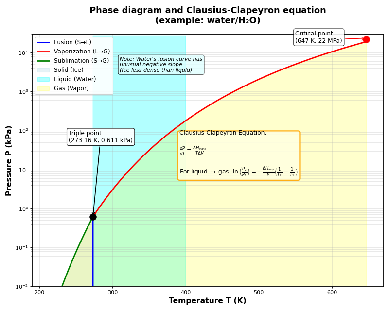

- How do you derive the Clausius-Clapeyron equation?
The Clausius-Clapeyron equation describes how vapor pressure changes with temperature during a phase transition. It starts from the equilibrium condition (see Gibbs free energy and volume for the derivation of \(dG\)).
Step 1: Start from equilibrium condition
At phase equilibrium (e.g., liquid-vapor), the Gibbs free energies of both phases are equal. As conditions change, they remain equal:
\[dG_{\text{liquid}} = dG_{\text{vapor}}\]From the previous derivation, \(dG = VdP - SdT\), so:
\[V_{\text{liquid}}dP - S_{\text{liquid}}dT = V_{\text{vapor}}dP - S_{\text{vapor}}dT\]Rearrange:
\[(V_{\text{vapor}} - V_{\text{liquid}})dP = (S_{\text{vapor}} - S_{\text{liquid}})dT\]Define \(\Delta \tilde{V} = V_{\text{vapor}} - V_{\text{liquid}}\) and \(\Delta S = S_{\text{vapor}} - S_{\text{liquid}}\):
\[\Delta \tilde{V} \, dP = \Delta S \, dT\]Therefore:
\[\frac{dP}{dT} = \frac{\Delta S}{\Delta \tilde{V}}\]Since \(\Delta S = \frac{\Delta H_{\text{vap}}}{T}\) at equilibrium (see Entropy change during phase transition):
\[\frac{dP}{dT} = \frac{\Delta H_{\text{vap}}}{T \Delta \tilde{V}}\]
Step 2: Simplify using ideal gas approximation
For liquid to vapor transition, the molar volume jump is dominated by the vapor. Here, \(\tilde{V}\) denotes molar volume (volume per mole):
\[\Delta \tilde{V} \approx \tilde{V}_g \approx \frac{RT}{P} \quad \text{(ideal gas)}\]where \(R\) is the gas constant, and the ideal gas law for one mole gives \(P\tilde{V} = RT\).
Step 3: Substitute and simplify
\[\frac{dP}{dT} = \frac{\Delta H_{\text{vap}}}{T} \cdot \frac{P}{RT} = \frac{\Delta H_{\text{vap}} \, P}{R \, T^2}\]
Step 4: Separate variables
\[\frac{1}{P} dP = \frac{\Delta H_{\text{vap}}}{R} \frac{1}{T^2} dT\]
Step 5: Integrate
Assuming \(\Delta H_{\text{vap}}\) is roughly constant over the temperature range:
\[\int_{P_1}^{P_2} \frac{1}{P} dP = \frac{\Delta H_{\text{vap}}}{R} \int_{T_1}^{T_2} \frac{1}{T^2} dT\]\[\ln\left(\frac{P_2}{P_1}\right) = \frac{\Delta H_{\text{vap}}}{R} \left[-\frac{1}{T}\right]_{T_1}^{T_2} = -\frac{\Delta H_{\text{vap}}}{R} \left(\frac{1}{T_2} - \frac{1}{T_1}\right)\]This is the Clausius-Clapeyron equation in integrated form. It relates vapor pressure at two different temperatures.
Example: Vapor pressure of water using Clausius-Clapeyron
Problem: Water has a vapor pressure of 1.00 atm at 100°C (373 K). The heat of vaporization is ΔH_vap = 40.66 kJ/mol. Calculate the vapor pressure at:
25°C (298 K)
120°C (393 K)
Solution:
Use the Clausius-Clapeyron equation:
Given: P₁ = 1.00 atm at T₁ = 373 K, ΔH_vap = 40,660 J/mol, R = 8.314 J/(mol·K)
Part 1: At 25°C (298 K)
Literature value: 23.8 mmHg (our calculation is within 18%, good for this approximation!)
Part 2: At 120°C (393 K)
Literature value: 1.99 atm (within 3%!)
Physical interpretation:
At lower temperature (25°C): Much lower vapor pressure because fewer molecules have enough energy to escape the liquid
At higher temperature (120°C): Higher vapor pressure, which is why pressure cookers work at elevated temperatures
Example: Measuring heat of vaporization experimentally
Problem: You measure the vapor pressure of ethanol at two temperatures: P₁ = 0.20 atm at T₁ = 40°C (313 K) and P₂ = 0.60 atm at T₂ = 60°C (333 K). Calculate ΔH_vap.
Solution:
Rearrange Clausius-Clapeyron to solve for ΔH_vap:
Literature value: 38.6 kJ/mol for ethanol (our value is ~23% high, suggesting the ideal gas approximation and constant ΔH_vap assumption have significant error)
Practical experimental setup:
Sealed container with ethanol and vapor space
Temperature control using water bath or heating mantle
Pressure gauge (manometer or digital sensor)
Equilibration time (wait for liquid-vapor equilibrium)
Plot ln P vs 1/T: The slope gives -ΔH_vap/R
This method allows determination of ΔH_vap without directly measuring heat transfer!
Nov 18, 2025 (Tue)
We are looking at a classic eutectic phase diagram for a binary mixture.
When you draw a vertical line across the eutetic point, how do you determine the composition?
What is the Gibb’s phase rule and how is it applied to phase diagrams?
What is the concept of solubility?
Congruent point?
Can you draw the G vs. composition at constant T?
How to determine phase compositions at a given temperature
In a binary phase diagram with components A and B, the total composition satisfies \(X_A + X_B = 1\), where \(X_A\) and \(X_B\) represent the mole fractions of each component. At any given temperature, the system may contain multiple phases (such as liquid, \(\alpha\) solid, and \(\beta\) solid), each with its own distinct composition. The procedure for determining these phase compositions uses the tie-line construction.
Step 1: Draw the tie line
Locate the temperature of interest on the vertical axis and draw a horizontal line (called a tie line) across the phase diagram. This line intersects the phase boundaries at points that define the compositions of coexisting phases.
Step 2: Read compositions from phase boundaries
At each intersection point between the tie line and a phase boundary, read the composition from the horizontal axis. These values give the compositions of the individual phases at equilibrium.
Example: Two-phase region with α and β
Consider a binary alloy at temperature \(T\) with overall composition \(X_0 = 0.40\) (40% B, 60% A). Suppose the tie line at this temperature intersects the phase boundaries at:
\(\alpha\) phase boundary: \(X_\alpha = 0.20\) (20% B in the \(\alpha\) solid)
\(\beta\) phase boundary: \(X_\beta = 0.70\) (70% B in the \(\beta\) solid)
The \(\alpha\) phase is A-rich (contains mostly A with some B dissolved), while the \(\beta\) phase is B-rich (contains mostly B with some A dissolved). The overall composition \(X_0 = 0.40\) lies between these two boundary values, confirming that both phases coexist at this temperature.
Step 3: Apply the lever rule to find phase fractions
The lever rule determines the relative amounts of each phase present. It works like a balance: the fraction of each phase is inversely proportional to the distance from the overall composition to that phase’s boundary composition.
Mathematically, the fractions are:
where \(f_\alpha + f_\beta = 1\) ensures mass conservation.
Derivation of the lever rule from mass balance
The lever rule is not arbitrary—it follows directly from conservation of mass (or moles) of component B. Consider a system with overall composition \(X_0\) that separates into two phases: \(\alpha\) with composition \(X_\alpha\) and \(\beta\) with composition \(X_\beta\).
Setup:
Consider 1 mole of total alloy (A + B combined). After equilibration at temperature \(T\), this alloy separates into two phases. Let \(f_\alpha\) represent the fraction (in moles) of the total alloy that becomes \(\alpha\) phase, and \(f_\beta\) represent the fraction that becomes \(\beta\) phase.
Since the phases must account for all the material:
This is Constraint 1: Total mass conservation. For example, if \(f_\alpha = 0.60\), then 0.60 moles of the original 1 mole alloy are in the \(\alpha\) phase, and 0.40 moles are in the \(\beta\) phase.
Constraint 2: Component B mass balance
Now track component B specifically. In the original 1 mole of alloy with composition \(X_0\), there are \(X_0\) moles of B (and \(1 - X_0\) moles of A).
After phase separation:
The \(\alpha\) phase (which is \(f_\alpha\) moles total) has composition \(X_\alpha\), so it contains \(f_\alpha \times X_\alpha\) moles of B
The \(\beta\) phase (which is \(f_\beta\) moles total) has composition \(X_\beta\), so it contains \(f_\beta \times X_\beta\) moles of B
The total B content must be unchanged (atoms don’t disappear):
Solve for phase fractions:
From Constraint 1: \(f_\beta = 1 - f_\alpha\)
Substitute into the B mass balance equation:
Expand:
Collect \(f_\alpha\) terms:
Solve for \(f_\alpha\):
Multiply numerator and denominator by -1 to get the standard form:
Similarly, solve for \(f_\beta\) using \(f_\alpha = 1 - f_\beta\):
Interpretation:
The numerator in each formula represents the “distance” from the overall composition to the opposite phase boundary:
\(f_\alpha\) fraction depends on distance \(|X_\beta - X_0|\) (distance to \(\beta\) boundary)
\(f_\beta\) fraction depends on distance \(|X_0 - X_\alpha|\) (distance to \(\alpha\) boundary)
The denominator \(|X_\beta - X_\alpha|\) is the total distance between the two phase boundaries (the length of the tie line).
This inverse relationship (farther boundary → smaller fraction) is exactly how a mechanical lever works: the fulcrum sits at \(X_0\), and the masses (phase fractions) balance according to their distances from the fulcrum.
Numerical example:
Using \(X_0 = 0.40\), \(X_\alpha = 0.20\), and \(X_\beta = 0.70\):
The system contains 60% \(\alpha\) phase and 40% \(\beta\) phase by mole fraction. Each phase’s fraction is proportional to the distance from the overall composition to the opposite boundary — this inverse relationship is why it is called the “lever” rule.
Congruent melting
- What is congruent melting?
Congruent melting occurs when a solid phase melts to produce a liquid with exactly the same composition as the solid.
Contrast with incongruent melting
Most compositions in a binary system exhibit incongruent melting: the solid melts over a temperature range, producing a liquid with a different composition than the starting solid. As temperature increases through the two-phase region, both the liquid composition and the relative amounts of solid and liquid change continuously.
For example, if you heat a solid with \(X_B = 0.25\) in the same A-B system:
At \(T_1\): Solid begins to melt, producing liquid with \(X_B = 0.40\) (different from solid)
During melting: Liquid composition gradually changes along the liquidus curve
At \(T_2\): Last bit of solid disappears, system becomes fully liquid
The liquid composition at the start of melting (\(X_B = 0.40\)) differs from the original solid composition (\(X_B = 0.25\)).
- Why do we care about congruent melting?
Congruent melting is important for several practical and theoretical reasons:
1. Crystal growth and materials synthesis
Compounds that melt congruently can be grown from their own melt without composition changes. This is crucial for:
Growing single crystals with precise stoichiometry
Avoiding compositional gradients during solidification
Producing phase-pure materials reproducibly
Example: Silicon melts congruently, allowing production of ultra-pure single crystals for semiconductors using the Czochralski process.
2. Identifying stable compounds
A congruent melting point indicates a thermodynamically stable compound at that composition. The compound is stable with respect to decomposition into neighboring phases up to its melting temperature.
In contrast, compounds that decompose before melting (peritectic decomposition) or melt incongruently are less stable.
3. Phase diagram topology
Congruent melting points divide a binary phase diagram into separate regions. Each congruent maximum acts like a “pseudo-pure component,” effectively breaking the diagram into simpler sub-systems that can be analyzed independently.
This simplifies understanding complex multi-component systems.
4. Processing temperature selection
For manufacturing, knowing whether a material melts congruently determines processing strategies:
Congruent: Can melt and refreeze repeatedly without composition drift
Incongruent: Melting causes phase separation, requiring careful temperature and composition control
Example: Stoichiometric compounds like \(\text{GaAs}\) (gallium arsenide) melt congruently at 1511 K, allowing direct melt growth. But if the composition is slightly off-stoichiometry, melting becomes incongruent and crystal quality suffers.
How to identify congruent melting on a phase diagram
Look for these features:
A peak (maximum or minimum) where liquidus and solidus meet at the same composition
A vertical line through this point indicates the composition melts at a single temperature
The phase boundary has \(dT/dX = 0\) at the congruent point (horizontal tangent)
At compositions away from the congruent point, the liquidus and solidus separate, creating a two-phase region where melting occurs over a temperature range.