Divergence measures how much a vector field spreads out or converges at a point. It’s a scalar quantity that describes the “source” or “sink” strength of the field.
Zero divergence: No net outflow (incompressible flow)
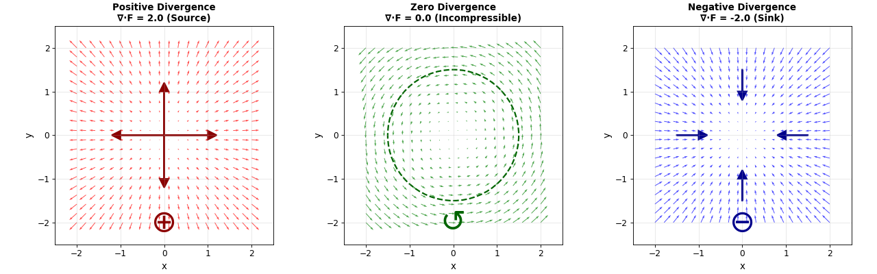
Visualization of positive, zero, and negative divergence:
The left panel shows positive divergence (source) for the vector field \(\mathbf{F} = (x, y)\), which has \(\nabla \cdot \mathbf{F} = +2\). Field lines radiate outward from the origin. The middle panel shows zero divergence for the rotational field \(\mathbf{F} = (-y, x)\), which has \(\nabla \cdot \mathbf{F} = 0\)—this is an incompressible flow where fluid circulates without expansion or compression. The right panel shows negative divergence (sink) for \(\mathbf{F} = (-x, -y)\), which has \(\nabla \cdot \mathbf{F} = -2\). Field lines converge toward the origin.
How to calculate divergence:
For the positive divergence case \(\mathbf{F} = (x, y)\):
Curl measures the rotation or circulation of a vector field. It’s a vector quantity that describes how much and in what direction the field “swirls” around a point.
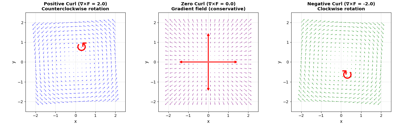
Visualization of positive, zero, and negative curl:
The left panel shows positive curl (counterclockwise rotation) for the vector field \(\mathbf{F} = (-y, x)\), which has \(\nabla \times \mathbf{F} = +2\). The middle panel shows zero curl for the gradient field \(\mathbf{F} = (2x, 2y) = \nabla(x^2 + y^2)\), which has \(\nabla \times \mathbf{F} = 0\)—this is a conservative field that can be integrated to give a scalar potential. The right panel shows negative curl (clockwise rotation) for \(\mathbf{F} = (y, -x)\), which has \(\nabla \times \mathbf{F} = -2\).
How to calculate curl in 2D:
In 2D, we only need the z-component of curl (the component pointing out of the page):
A conservative field is a vector field that can be written as the gradient of a scalar function (potential). If \(\mathbf{F} = \nabla \phi\) for some scalar \(\phi\), then the field is conservative.
Key property: The curl of any gradient is zero:
\[\nabla \times (\nabla \phi) = \mathbf{0}\]
This works both ways:
Forward: If you have a scalar function \(\phi(x,y)\), its gradient \(\nabla \phi = (\partial \phi/\partial x, \partial \phi/\partial y)\) gives you a vector field with zero curl
Backward (integration): If you have a vector field with zero curl, you can integrate it to find the original scalar function \(\phi\)
Example from the middle panel:
Start with scalar: \(\phi(x,y) = x^2 + y^2\)
Take gradient: \(\nabla \phi = (2x, 2y)\) — this is the vector field (arrows pointing outward)
Check curl: \(\nabla \times (2x, 2y) = \partial(2y)/\partial x - \partial(2x)/\partial y = 0 - 0 = 0\) ✓
Why “conservative”? The term comes from physics—specifically from the conservation of mechanical energy. When a force field is conservative, the total mechanical energy (kinetic + potential) remains constant as you move through the field.
The physics origin:
When you move an object through a force field \(\mathbf{F}\) from point A to point B, the work done is:
\[W = \int_A^B \mathbf{F} \cdot d\mathbf{r}\]
For a conservative field where \(\mathbf{F} = -\nabla U\) (force is negative gradient of potential energy \(U\)):
The work depends only on the start and end points, not on the path taken. This means:
Closed path work is zero: If you return to your starting point (A = B), then \(W = U_A - U_A = 0\). No net energy is gained or lost going around a loop.
Energy is conserved: The work done by the force equals the decrease in potential energy, so \(E_{\text{kinetic}} + U = \text{constant}\).
Path independence: You can take any route from A to B and do the same amount of work.
Examples of conservative forces:
Gravity: \(\mathbf{F} = -mg\mathbf{\hat{z}}\), potential \(U = mgz\). Lifting an object 10 meters requires the same energy whether you go straight up or spiral around.
Electrostatic: \(\mathbf{F} = k\frac{q_1 q_2}{r^2}\mathbf{\hat{r}}\), potential \(U = k\frac{q_1 q_2}{r}\). Moving a charge in an electric field conserves energy.
Spring force: \(\mathbf{F} = -kx\mathbf{\hat{x}}\), potential \(U = \frac{1}{2}kx^2\). Compressing a spring stores energy that can be fully recovered.
Non-conservative forces:
Friction: Sliding an object around a loop dissipates energy as heat. The work depends on path length, not just endpoints. Cannot be written as \(\mathbf{F} = -\nabla U\).
Magnetic force: \(\mathbf{F} = q\mathbf{v} \times \mathbf{B}\). Always perpendicular to motion, does zero work, but still has curl (circulation around magnetic field lines).
Why curl = 0 for conservative fields?
If \(\mathbf{F} = -\nabla U\), then by the vector calculus identity \(\nabla \times (\nabla U) = \mathbf{0}\), the curl must be zero. Physically, curl represents circulation or rotation in the field. If there’s circulation, you can extract energy by going around a loop (like a water wheel in a vortex), violating energy conservation.
Connection to DPC: When you measure center of mass shifts \((g_x, g_y)\) in DPC, you’re measuring the gradient of the phase \(\nabla \phi\). If curl is zero, you can integrate \(g_x\) and \(g_y\) to recover the original phase \(\phi(x,y)\). If curl is non-zero, the field is not conservative and integration gives inconsistent results (you can’t find a single-valued \(\phi\)).
Why is curl important in DPC?
In Differential Phase Contrast (DPC) microscopy, we measure the center of mass shift vector field \(\mathbf{g}(r_x, r_y) = (\text{com}_x, \text{com}_y)\). This vector field should ideally be the gradient of a scalar phase:
This is because the curl of a gradient is always zero:
\[\nabla \times (\nabla f) = \mathbf{0}\]
This is a fundamental vector calculus identity: the curl of any conservative vector field (one that can be written as the gradient of a function) is zero.
What does it mean when curl is not zero in DPC?
When \(\nabla \times \mathbf{g} \neq 0\), the measured center of mass field is not conservative—it cannot be perfectly integrated to give a single-valued phase. This happens due to:
Measurement noise: Random errors in center of mass detection
Sample rotation: Physical misalignment between scan and detector coordinates
Software like Ophus computes the curl and finds the optimal rotation angle where \(\nabla \times \mathbf{g}\) becomes minimized. This aligns the coordinate systems and removes systematic errors before phase integration.
What is the phase from electrostatic potential?
The phase shift acquired by an electron passing through an electrostatic potential \(V(x,y,z)\) is:
\[\phi(x,y) = \sigma \int V(x,y,z)\,dz\]
where \(\sigma\) is the interaction constant. This is the real-space reconstructed phase image that relates to the sample’s potential.
“Phase contrast” means large \(\phi\) corresponds to regions with stronger potential (higher atomic number \(Z\) or greater thickness).
Properties of divergence and curl summary
Key identities:
\(\nabla \times (\nabla f) = \mathbf{0}\) — curl of a gradient is zero
\(\nabla \cdot (\nabla \times \mathbf{F}) = 0\) — divergence of a curl is zero
If \(\nabla \times \mathbf{F} = \mathbf{0}\) everywhere, then \(\mathbf{F} = \nabla \phi\) for some scalar \(\phi\) (conservative field)
These identities are fundamental to understanding why DPC works: we measure gradients (center of mass shifts) and integrate them back to get phase, but this only works perfectly when curl is zero.
The Laplacian measures the curvature of a function. It quantifies how much a function’s value at a point differs from the average of its neighbors. The Laplacian is the divergence of the gradient:
\[\nabla \cdot \nabla f = \nabla^2 f = \frac{\partial^2 f}{\partial x^2} + \frac{\partial^2 f}{\partial y^2} + \frac{\partial^2 f}{\partial z^2}\]
Physical interpretation:
Positive Laplacian: Function curves upward (like a bowl), value is below its neighbors
Negative Laplacian: Function curves downward (like a peak), value is above its neighbors
Zero Laplacian: Function is at equilibrium with its neighbors (harmonic function)
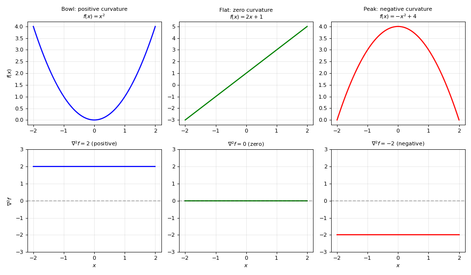
How does the Laplacian measure curvature?
The Laplacian detects how a surface bends. This curvature information encodes how the function differs from a flat plane at each point.
The top row shows three functions with different curvatures. The bottom row shows their Laplacian values. A bowl curves upward (positive Laplacian), a flat line has no curvature (zero Laplacian), and a peak curves downward (negative Laplacian).
The discrete approximation (finite differences):
On a computational grid, the Laplacian is approximated using neighboring points. For a 1D function \(u(x)\) at grid point \(x_i\):
The five-point stencil is like a tiny compass that checks the function in four cardinal directions (left, right, up, down) and compares them to the center. This comparison encodes how the surface bends locally.
Geometric interpretation:
Curvature is what the Laplacian measures. The symmetric “plus” shape captures this by averaging differences in perpendicular directions:
Each second derivative\(\partial^2 u/\partial x^2\) and \(\partial^2 u/\partial y^2\) measures bending in one direction
Adding them gives total curvature in all directions
The pattern is almost like a tiny compass that checks if the value at a point differs from the average of its four neighbors.
How does the 2D Laplacian work?
The 2D generalization extends the same idea to a grid. At each grid point \((i,j)\), the Laplacian is:
\[\Delta u = \frac{\partial^2 u}{\partial x^2} + \frac{\partial^2 u}{\partial y^2}\]
Each second derivative gets its own copy of the 1D finite-difference formula. If grid spacing is \(h\):
The negative Laplacian (-4.0) indicates the center value (3.0) is above the average of its four neighbors (all 2.0), forming a local peak. If this were a temperature distribution, heat would flow away from the center since it’s hotter than its surroundings.
How do NumPy and SciPy calculate the Laplacian?
In practice, NumPy and SciPy use the five-point stencil method described above. The most common functions are:
scipy.ndimage.laplace:
fromscipy.ndimageimportlaplaceimportnumpyasnp# Create a 2D arrayu=np.array([[1.0,2.0,1.0],[2.0,3.0,2.0],[1.0,2.0,1.0]])# Compute Laplacianlaplacian=laplace(u)# Result at center: -4.0
This function applies the five-point stencil to every interior point. Edge points use boundary conditions (default is reflecting).
Manual convolution with kernel:
The Laplacian can also be computed as a convolution with a kernel:
This kernel directly encodes the formula: \(u_{i-1,j} + u_{i+1,j} + u_{i,j-1} + u_{i,j+1} - 4u_{i,j}\).
When to use nine-point stencil:
The five-point stencil is accurate and numerically stable for most applications. However, a nine-point stencil can be preferred in specific cases:
# Nine-point stencil (more accurate, more isotropic)kernel=np.array([[1,4,1],[4,-20,4],[1,4,1]])/6.0
Advantages of nine-point stencil:
Better isotropy: The five-point stencil has directional bias (only samples along axes). The nine-point stencil includes diagonals, making it more rotationally symmetric.
Higher accuracy: Fourth-order accurate on smooth functions versus second-order for five-point.
Better for anisotropic grids: When grid spacing differs in x and y directions.
When five-point is sufficient:
The five-point stencil is the standard choice for:
Regular grids with uniform spacing
Fast computation (fewer operations)
Most physics simulations (heat, wave equations)
Image processing where isotropy is less critical
The five-point stencil is not inherently unstable. Both stencils are stable for typical applications. The nine-point stencil is chosen for accuracy and isotropy, not stability.
Why is the Laplacian important?
The Laplacian appears throughout physics and mathematics because it naturally describes how systems evolve toward equilibrium:
The kinetic energy term involves the Laplacian of the wavefunction.
Connection to phase retrieval
In electron microscopy, the phase \(\phi(x,y)\) relates to the sample’s electrostatic potential. The Laplacian of the phase encodes information about charge distribution and local curvature in the projected potential. Phase retrieval methods often use regularization terms involving \(\nabla^2 \phi\) to ensure smooth, physically reasonable reconstructions.
Integration by parts is a technique for evaluating integrals that involve products of functions. It transfers a derivative from one function to another at the cost of a boundary term and a sign flip. The formula is:
This is the integration by parts formula. It shows that integrating \(u'(x) v(x)\) is equivalent to integrating \(u(x) v'(x)\) with opposite sign, plus a boundary term.
Alternative notation
Using differential notation \(du = u'(x)\,dx\) and \(dv = v'(x)\,dx\), the formula becomes:
\[\int u \, dv = uv - \int v \, du\]
This compact form is commonly used in calculus textbooks.
Example: Computing\(\int x e^x \, dx\)
Choose \(u = x\) (which simplifies when differentiated) and \(dv = e^x dx\) (which stays simple when integrated):
\(u = x\) → \(du = dx\)
\(dv = e^x dx\) → \(v = e^x\)
Apply integration by parts:
\[\int x e^x \, dx = x e^x - \int e^x \, dx = x e^x - e^x + C = e^x(x - 1) + C\]
The technique converted a product integral into a simpler integral.
Example: Computing\(\int \ln(x) \, dx\)
This looks like a single function, but treat it as \(\ln(x) \cdot 1\). Choose \(u = \ln(x)\) (simplifies when differentiated) and \(dv = dx\):
\(u = \ln(x)\) → \(du = \frac{1}{x} dx\)
\(dv = dx\) → \(v = x\)
Apply integration by parts:
\[\int \ln(x) \, dx = x \ln(x) - \int x \cdot \frac{1}{x} \, dx = x \ln(x) - \int 1 \, dx = x \ln(x) - x + C\]
Without integration by parts, this integral would be difficult to evaluate directly.
A Taylor series represents a function as an infinite sum of polynomial terms, each derived from the function’s derivatives at a single point. For a function \(f(x)\) expanded around point \(a\), the Taylor series is:
The exact value is \(\sin(0.1) = 0.0998334...\), so the error is only \(4 \times 10^{-7}\) (0.0004%). Just three terms give excellent accuracy near the expansion point.
Numerical example 2: Point far from the expansion point
Approximate \(\sin(3)\) using the same order-3 Taylor series around \(a = 0\):
The exact value is \(\sin(3) = 0.14112...\), so the approximation gives \(-1.5\) (completely wrong!). The error is enormous because \(x = 3\) radians is far from the expansion point \(a = 0\).
To get accuracy at \(x = 3\), either:
Use many more terms (order 7 gives \(0.091\), order 15 gives \(0.141\), nearly exact)
Expand around a different point closer to \(x = 3\), like \(a = \pi \approx 3.14\)
Numerical example 3: Expanding around\(a = \pi\)instead
To approximate \(\sin(3)\) more accurately, expand around \(a = \pi \approx 3.14159\) (which is close to \(x = 3\)).
The exact value is \(\sin(3) = 0.14112\), so the approximation matches to 5 decimal places! By choosing \(a = \pi\) close to \(x = 3\), just three terms give excellent accuracy.
Key insight: Choosing the right expansion point \(a\) near the target \(x\) is often more effective than adding many terms to a distant expansion.
Physical interpretation
The Taylor series approximates a function using only local information at point \(a\). Each term adds more accuracy:
Zeroth order (\(f(a)\)): Constant approximation
First order (\(f(a) + f'(a)(x-a)\)): Linear approximation (tangent line)
Second order: Adds quadratic curvature
Third order: Adds cubic bending
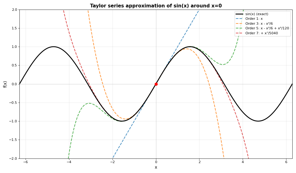
Near \(x = a\), the series converges rapidly. Far from \(a\), more terms are needed for accuracy.
The plot shows how higher-order Taylor polynomials progressively match \(\sin(x)\) over a wider range. Near \(x = 0\), even the linear approximation (\(f(x) \approx x\)) is quite good. Far from the expansion point, higher-order terms are essential.
For small values of \(x\) (typically \(|x| \ll 1\)), higher-order terms in Taylor series become negligible. Keeping only the first few terms gives simple approximations used throughout physics and engineering.
Small-angle approximation for sine:
\[\sin(x) \approx x \quad \text{for } |x| \ll 1\]
This is the first-order Taylor approximation. The error is \(O(x^3)\), meaning if \(x = 0.1\), the error is roughly \(x^3/6 \approx 0.000167\).
Example:\(\sin(0.1) = 0.0998334...\) while the approximation gives \(0.1\), an error of only 0.17%.