Quantum mechanics II

Note

This page continues from Quantum mechanics I. Make sure you’re familiar with wave-particle duality, the Schru00f6dinger equation, hydrogen atom, angular momentum, spin, and mathematical foundations before proceeding.

The particle in a box taught us about discrete energy levels and standing waves, but the infinite walls were artificial. What happens when we have a more realistic potential? The quantum harmonic oscillator is the next essential system to master. Unlike the box with its abrupt infinite walls, the harmonic oscillator has a smooth parabolic potential that appears everywhere in nature: vibrating molecules, atoms in solids, photons in cavities, and even quantum fields themselves. Moreover, we will solve this problem using a completely different technique (ladder operators) that reveals deep connections to quantum field theory and introduces the concept of particle creation and annihilation.

Quantum harmonic oscillator

The problem setup

What is the harmonic oscillator potential?

A particle experiences a restoring force proportional to its displacement from equilibrium, like a mass on a spring:

\[F = -kx \quad \Rightarrow \quad V(x) = \frac{1}{2}kx^2 = \frac{1}{2}m\omega^2 x^2\]

where:

\(k\): spring constant
\(\omega = \sqrt{k/m}\): angular frequency
\(m\): particle mass

Physical examples:

Vibrating diatomic molecules (atoms connected by chemical bonds)
Lattice vibrations in solids (phonons)
Light modes in optical cavities (photons)
Quantum field theory (field excitations)

Why is this problem important?

The harmonic oscillator is fundamental in physics because:

Universal approximation: Any smooth potential near a minimum looks like \(V \approx V_0 + \frac{1}{2}k(x-x_0)^2\)
Exactly solvable: One of the few quantum problems with analytical solutions
Basis for perturbation theory: Small deviations from harmonic behavior can be treated as perturbations
Foundation of quantum field theory: Creation and annihilation operators originated here

The time-independent Schrödinger equation

What equation do we need to solve?

For the harmonic oscillator potential, the time-independent Schrödinger equation is:

\[-\frac{\hbar^2}{2m} \frac{d^2\psi}{dx^2} + \frac{1}{2}m\omega^2 x^2 \psi = E \psi\]

This is a second-order differential equation. Unlike the particle in a box, we cannot use simple sine and cosine functions because the potential varies with position.

Boundary conditions: As \(x \to \pm\infty\), we require \(\psi \to 0\) (normalization).

The problem with the direct approach

Why not just solve the differential equation?

Solving this differential equation directly is algebraically tedious:

Transform to dimensionless variables: \(\xi = \sqrt{m\omega/\hbar} \, x\)
Analyze asymptotic behavior as \(\xi \to \pm\infty\)
Find polynomial solutions that ensure normalizability
Apply boundary conditions to determine allowed energies

This works, but requires advanced techniques involving special functions. There must be a better way!

Solving with ladder operators

The elegant algebraic approach

Instead of solving the differential equation, we use ladder operators (also called creation and annihilation operators). This algebraic method:

Avoids differential equations entirely: Pure operator algebra
Reveals why energy levels are equally spaced: Direct consequence of commutation relations
Finds all states efficiently: Generate entire spectrum from ground state
Generalizes to other problems: Same technique works for angular momentum, quantum field theory

This is the standard modern approach to the harmonic oscillator!

Defining the ladder operators

We define two operators from position \(\hat{x}\) and momentum \(\hat{p}\):

\[\hat{a} = \sqrt{\frac{m\omega}{2\hbar}} \hat{x} + i\frac{\hat{p}}{\sqrt{2m\hbar\omega}}\]

\[\hat{a}^\dagger = \sqrt{\frac{m\omega}{2\hbar}} \hat{x} - i\frac{\hat{p}}{\sqrt{2m\hbar\omega}}\]

where \(\hat{a}\) is the lowering operator (annihilation) and \(\hat{a}^\dagger\) is the raising operator (creation).

Rewriting the Hamiltonian using ladder operators

How do we express the Hamiltonian in terms of ladder operators?

Start with the classical Hamiltonian:

\[\hat{H} = \frac{\hat{p}^2}{2m} + \frac{1}{2}m\omega^2 \hat{x}^2\]

Goal: Rewrite this using \(\hat{a}\) and \(\hat{a}^\dagger\).

Step 1: Express position and momentum in terms of ladder operators

From the definitions of \(\hat{a}\) and \(\hat{a}^\dagger\), we can solve for \(\hat{x}\) and \(\hat{p}\).

Results:

\[\boxed{\hat{x} = \sqrt{\frac{\hbar}{2m\omega}} (\hat{a}^\dagger + \hat{a})}\]

\[\boxed{\hat{p} = i\sqrt{\frac{m\hbar\omega}{2}} (\hat{a}^\dagger - \hat{a})}\]

Step 2: Calculate \(\hat{x}^2\)

\[\hat{x}^2 = \frac{\hbar}{2m\omega} (\hat{a}^\dagger + \hat{a})^2 = \frac{\hbar}{2m\omega} (\hat{a}^\dagger \hat{a}^\dagger + \hat{a}^\dagger \hat{a} + \hat{a}\hat{a}^\dagger + \hat{a}\hat{a})\]

Step 3: Calculate \(\hat{p}^2\)

\[\hat{p}^2 = -\frac{m\hbar\omega}{2} (\hat{a}^\dagger - \hat{a})^2 = -\frac{m\hbar\omega}{2} (\hat{a}^\dagger \hat{a}^\dagger - \hat{a}^\dagger \hat{a} - \hat{a}\hat{a}^\dagger + \hat{a}\hat{a})\]

Step 4: Substitute into the Hamiltonian

\[\hat{H} = \frac{\hat{p}^2}{2m} + \frac{1}{2}m\omega^2 \hat{x}^2\]

\[= \frac{1}{2m}\left[-\frac{m\hbar\omega}{2} (\hat{a}^\dagger \hat{a}^\dagger - \hat{a}^\dagger \hat{a} - \hat{a}\hat{a}^\dagger + \hat{a}\hat{a})\right] + \frac{1}{2}m\omega^2 \left[\frac{\hbar}{2m\omega} (\hat{a}^\dagger \hat{a}^\dagger + \hat{a}^\dagger \hat{a} + \hat{a}\hat{a}^\dagger + \hat{a}\hat{a})\right]\]

Simplify:

\[= -\frac{\hbar\omega}{4} (\hat{a}^\dagger \hat{a}^\dagger - \hat{a}^\dagger \hat{a} - \hat{a}\hat{a}^\dagger + \hat{a}\hat{a}) + \frac{\hbar\omega}{4} (\hat{a}^\dagger \hat{a}^\dagger + \hat{a}^\dagger \hat{a} + \hat{a}\hat{a}^\dagger + \hat{a}\hat{a})\]

Step 5: Collect terms

Notice the \(\hat{a}^\dagger \hat{a}^\dagger\) terms cancel, the \(\hat{a}\hat{a}\) terms cancel, and we’re left with:

\[\hat{H} = \frac{\hbar\omega}{4} (\hat{a}^\dagger \hat{a} + \hat{a}\hat{a}^\dagger + \hat{a}^\dagger \hat{a} + \hat{a}\hat{a}^\dagger)\]

\[= \frac{\hbar\omega}{4} (2\hat{a}^\dagger \hat{a} + 2\hat{a}\hat{a}^\dagger)\]

\[= \frac{\hbar\omega}{2} (\hat{a}^\dagger \hat{a} + \hat{a}\hat{a}^\dagger)\]

Step 6: Use the commutation relation

We need the commutation relation \([\hat{a}, \hat{a}^\dagger] = 1\), which means \(\hat{a}\hat{a}^\dagger = \hat{a}^\dagger \hat{a} + 1\).

Substitute \(\hat{a}\hat{a}^\dagger = \hat{a}^\dagger \hat{a} + 1\):

\[\hat{H} = \frac{\hbar\omega}{2} (\hat{a}^\dagger \hat{a} + \hat{a}^\dagger \hat{a} + 1) = \frac{\hbar\omega}{2} (2\hat{a}^\dagger \hat{a} + 1)\]

\[\boxed{\hat{H} = \hbar\omega\left(\hat{a}^\dagger \hat{a} + \frac{1}{2}\right)}\]

Define the number operator

We’ve just shown that the Hamiltonian can be written as:

\[\hat{H} = \hbar\omega\left(\hat{a}^\dagger \hat{a} + \frac{1}{2}\right)\]

The problem we need to solve: We want to find the allowed energy levels. To do this, we need to solve the eigenvalue equation:

\[\hat{H}|\psi\rangle = E|\psi\rangle\]

But solving this directly is hard! Instead, we’ll use a clever trick involving the combination \(\hat{a}^\dagger \hat{a}\).

The number operator: solving the energy eigenvalue problem

Define the number operator:

\[\boxed{\hat{N} = \hat{a}^\dagger \hat{a}}\]

Then the Hamiltonian becomes:

\[\hat{H} = \hbar\omega\left(\hat{N} + \frac{1}{2}\right)\]

Key idea: If we can find the eigenstates and eigenvalues of \(\hat{N}\), we automatically get the energy eigenvalues!

Here’s why: Suppose \(|\psi\rangle\) is an eigenstate of \(\hat{N}\) with eigenvalue \(\lambda\):

\[\hat{N}|\psi\rangle = \lambda|\psi\rangle\]

Then applying the Hamiltonian:

\[\hat{H}|\psi\rangle = \hbar\omega\left(\hat{N} + \frac{1}{2}\right)|\psi\rangle = \hbar\omega\left(\lambda + \frac{1}{2}\right)|\psi\rangle\]

So the energy eigenvalue is \(E = \hbar\omega(\lambda + 1/2)\).

The problem reduced: Instead of solving for \(\hat{H}\), we just need to find the eigenvalues of \(\hat{N}\).

How N̂ works with â and â†: the key commutators

The magic of \(\hat{N}\) comes from how it commutes with the ladder operators.

Deriving \([\hat{N}, \hat{a}^\dagger]\):

Start with the commutator definition:

\[[\hat{N}, \hat{a}^\dagger] = \hat{N}\hat{a}^\dagger - \hat{a}^\dagger\hat{N}\]

Substitute \(\hat{N} = \hat{a}^\dagger \hat{a}\):

\[= (\hat{a}^\dagger \hat{a})\hat{a}^\dagger - \hat{a}^\dagger(\hat{a}^\dagger \hat{a})\]

Use associativity to regroup the first term:

\[= \hat{a}^\dagger (\hat{a}\hat{a}^\dagger) - \hat{a}^\dagger(\hat{a}^\dagger \hat{a})\]

Now use \(\hat{a}\hat{a}^\dagger = \hat{a}^\dagger \hat{a} + 1\):

\[= \hat{a}^\dagger (\hat{a}^\dagger \hat{a} + 1) - \hat{a}^\dagger(\hat{a}^\dagger \hat{a})\]

Distribute:

\[= \hat{a}^\dagger \hat{a}^\dagger \hat{a} + \hat{a}^\dagger - \hat{a}^\dagger \hat{a}^\dagger \hat{a}\]

The first and third terms cancel:

\[\boxed{[\hat{N}, \hat{a}^\dagger] = \hat{a}^\dagger}\]

Deriving \([\hat{N}, \hat{a}]\):

Start with:

\[[\hat{N}, \hat{a}] = \hat{N}\hat{a} - \hat{a}\hat{N}\]

Substitute \(\hat{N} = \hat{a}^\dagger \hat{a}\):

\[= (\hat{a}^\dagger \hat{a})\hat{a} - \hat{a}(\hat{a}^\dagger \hat{a})\]

Regroup the second term:

\[= \hat{a}^\dagger (\hat{a}\hat{a}) - (\hat{a}\hat{a}^\dagger) \hat{a}\]

Use \(\hat{a}\hat{a}^\dagger = \hat{a}^\dagger \hat{a} + 1\):

\[= \hat{a}^\dagger \hat{a}\hat{a} - (\hat{a}^\dagger \hat{a} + 1) \hat{a}\]

Distribute:

\[= \hat{a}^\dagger \hat{a}\hat{a} - \hat{a}^\dagger \hat{a}\hat{a} - \hat{a}\]

The first two terms cancel:

\[\boxed{[\hat{N}, \hat{a}] = -\hat{a}}\]

What do these commutators actually mean?

Understanding commutators: When \([\hat{A}, \hat{B}] = \hat{C}\), it means:

\[\hat{A}\hat{B} = \hat{B}\hat{A} + \hat{C}\]

So \([\hat{N}, \hat{a}^\dagger] = \hat{a}^\dagger\) means:

\[\hat{N}\hat{a}^\dagger = \hat{a}^\dagger \hat{N} + \hat{a}^\dagger\]

And \([\hat{N}, \hat{a}] = -\hat{a}\) means:

\[\hat{N}\hat{a} = \hat{a}\hat{N} - \hat{a}\]

Why does this matter? These relations tell us what happens when we apply \(\hat{N}\) after applying a ladder operator.

Key insight: If we have a state where we know the eigenvalue of \(\hat{N}\), these commutators tell us the eigenvalue of the new state after applying \(\hat{a}^\dagger\) or \(\hat{a}\).

Let’s see this in action in the next section!

Building the energy ladder

Suppose we have a state \(|n\rangle\) that satisfies:

\[\hat{N}|n\rangle = n|n\rangle\]

This means \(|n\rangle\) is an eigenstate of \(\hat{N}\) with eigenvalue \(n\).

Question: What happens when we apply \(\hat{a}^\dagger\) to this state? Is \(\hat{a}^\dagger|n\rangle\) also an eigenstate of \(\hat{N}\)? If so, what’s its eigenvalue?

Showing that â†|n⟩ is an eigenstate with eigenvalue n+1

Apply \(\hat{N}\) to the state \(\hat{a}^\dagger|n\rangle\).

We want to calculate \(\hat{N}(\hat{a}^\dagger|n\rangle)\). Start by writing it out:

\[\hat{N}(\hat{a}^\dagger |n\rangle)\]

Regroup the parentheses.

When we have multiple operators acting on a state, it doesn’t matter how we group them with parentheses. This property is called associativity. It means:

\[\hat{A}(\hat{B}|c\rangle) = (\hat{A}\hat{B})|c\rangle\]

Both expressions mean “first apply \(\hat{B}\) to the state, then apply \(\hat{A}\) to the result.” We can regroup:

\[= (\hat{N}\hat{a}^\dagger)|n\rangle\]

Now we need to figure out what \(\hat{N}\hat{a}^\dagger\) equals.

Use the commutator relation \([\hat{N}, \hat{a}^\dagger] = \hat{a}^\dagger\).

Recall that \([\hat{N}, \hat{a}^\dagger] = \hat{a}^\dagger\) means:

\[\hat{N}\hat{a}^\dagger - \hat{a}^\dagger\hat{N} = \hat{a}^\dagger\]

Rearrange to solve for \(\hat{N}\hat{a}^\dagger\):

\[\hat{N}\hat{a}^\dagger = \hat{a}^\dagger\hat{N} + \hat{a}^\dagger\]

Substitute this back into our expression:

\[(\hat{N}\hat{a}^\dagger)|n\rangle = (\hat{a}^\dagger\hat{N} + \hat{a}^\dagger)|n\rangle\]

Distribute over the state:

\[= \hat{a}^\dagger\hat{N}|n\rangle + \hat{a}^\dagger|n\rangle\]

Use the fact that \(\hat{N}|n\rangle = n|n\rangle\).

Substitute the eigenvalue equation:

\[= \hat{a}^\dagger(n|n\rangle) + \hat{a}^\dagger|n\rangle\]

Pull out the scalar \(n\) (numbers can move past operators):

\[= n(\hat{a}^\dagger|n\rangle) + \hat{a}^\dagger|n\rangle\]

Factor out the common term \(\hat{a}^\dagger|n\rangle\):

\[= (n + 1)(\hat{a}^\dagger|n\rangle)\]

Interpret the result.

We’ve shown that:

\[\hat{N}(\hat{a}^\dagger|n\rangle) = (n+1)(\hat{a}^\dagger|n\rangle)\]

This is exactly the eigenvalue equation! It says \(\hat{a}^\dagger|n\rangle\) is an eigenstate of \(\hat{N}\) with eigenvalue \(n+1\).

Conclusion:

\[\boxed{\hat{a}^\dagger |n\rangle \propto |n+1\rangle}\]

The \(\propto\) symbol means “proportional to” (they differ by a normalization constant). The key point: \(\hat{a}^\dagger\) increases the eigenvalue by 1!

Showing that â|n⟩ is an eigenstate with eigenvalue n-1

Now let’s do the same thing for \(\hat{a}\).

Apply \(\hat{N}\) to the state \(\hat{a}|n\rangle\):

\[\hat{N}(\hat{a}|n\rangle)\]

Regroup the parentheses (using associativity):

\[= (\hat{N}\hat{a})|n\rangle\]

Use the commutator relation \([\hat{N}, \hat{a}] = -\hat{a}\).

Recall that \([\hat{N}, \hat{a}] = -\hat{a}\) means:

\[\hat{N}\hat{a} - \hat{a}\hat{N} = -\hat{a}\]

Rearrange to solve for \(\hat{N}\hat{a}\):

\[\hat{N}\hat{a} = \hat{a}\hat{N} - \hat{a}\]

Substitute this back:

\[(\hat{N}\hat{a})|n\rangle = (\hat{a}\hat{N} - \hat{a})|n\rangle\]

Distribute over the state:

\[= \hat{a}\hat{N}|n\rangle - \hat{a}|n\rangle\]

Use \(\hat{N}|n\rangle = n|n\rangle\):

\[= \hat{a}(n|n\rangle) - \hat{a}|n\rangle\]

Pull out the scalar \(n\):

\[= n(\hat{a}|n\rangle) - \hat{a}|n\rangle\]

Factor out \(\hat{a}|n\rangle\):

\[= (n - 1)(\hat{a}|n\rangle)\]

Interpret the result.

We’ve shown that:

\[\hat{N}(\hat{a}|n\rangle) = (n-1)(\hat{a}|n\rangle)\]

This means \(\hat{a}|n\rangle\) is an eigenstate of \(\hat{N}\) with eigenvalue \(n-1\).

Conclusion:

\[\boxed{\hat{a}|n\rangle \propto |n-1\rangle}\]

The \(\hat{a}\) operator decreases the eigenvalue by 1!

Why they’re called ladder operators

Summary of what we just proved:

\(\hat{a}^\dagger\) raises the \(\hat{N}\) eigenvalue by 1: \(|n\rangle \xrightarrow{\hat{a}^\dagger} |n+1\rangle\)

\(\hat{a}\) lowers the \(\hat{N}\) eigenvalue by 1: \(|n\rangle \xrightarrow{\hat{a}} |n-1\rangle\)

This is like climbing up and down a ladder! Each “rung” of the ladder corresponds to a different value of \(n\).

Exact action of ladder operators with normalization

We’ve shown that \(\hat{a}^\dagger|n\rangle \propto |n+1\rangle\) and \(\hat{a}|n\rangle \propto |n-1\rangle\). But what are the exact proportionality constants?

For the raising operator:

We need to find the constant \(c_n\) such that:

\[\hat{a}^\dagger |n\rangle = c_n |n+1\rangle\]

To find \(c_n\), compute the norm of both sides.

Take the inner product \(\langle n | \hat{a} \hat{a}^\dagger | n \rangle\):

\[\langle n | \hat{a} \hat{a}^\dagger | n \rangle = |c_n|^2 \langle n+1 | n+1 \rangle = |c_n|^2\]

Now use the commutator \(\hat{a}\hat{a}^\dagger = \hat{a}^\dagger \hat{a} + 1\):

\[\langle n | \hat{a} \hat{a}^\dagger | n \rangle = \langle n | (\hat{a}^\dagger \hat{a} + 1) | n \rangle\]

\[= \langle n | \hat{a}^\dagger \hat{a} | n \rangle + \langle n | n \rangle\]

\[= \langle n | \hat{N} | n \rangle + 1 = n + 1\]

Therefore \(|c_n|^2 = n+1\), so:

\[\boxed{\hat{a}^\dagger |n\rangle = \sqrt{n+1} |n+1\rangle}\]

For the lowering operator:

Similarly, let \(\hat{a}|n\rangle = d_n |n-1\rangle\). Then:

\[\langle n | \hat{a}^\dagger \hat{a} | n \rangle = |d_n|^2\]

But \(\hat{a}^\dagger \hat{a} = \hat{N}\):

\[\langle n | \hat{N} | n \rangle = n\]

So \(|d_n|^2 = n\), giving:

\[\boxed{\hat{a}|n\rangle = \sqrt{n} |n-1\rangle}\]

Key results:

\[\hat{a}^\dagger |n\rangle = \sqrt{n+1} |n+1\rangle\]

\[\hat{a}|n\rangle = \sqrt{n} |n-1\rangle\]

Special case: For the ground state:

\[\hat{a}|0\rangle = \sqrt{0} |-1\rangle = 0\]

This confirms our earlier statement that \(\hat{a}|0\rangle = 0\).

Finding the ground state

Why must there be a ground state?

Energies must be bounded below, otherwise the system would be unphysical (could extract infinite energy). As we repeatedly apply \(\hat{a}\) to lower the energy, we must eventually reach a state that cannot be lowered further.

Defining the ground state:

The ground state \(|0\rangle\) is defined by the condition:

\[\hat{a}|0\rangle = 0\]

This is the ground state. For this state:

\[\hat{N}|0\rangle = \hat{a}^\dagger \hat{a}|0\rangle = \hat{a}^\dagger (0) = 0\]

So the ground state has \(n = 0\), giving energy:

\[E_0 = \hbar\omega\left(0 + \frac{1}{2}\right) = \frac{1}{2}\hbar\omega\]

Building all states

Starting from \(|0\rangle\), we can build all excited states:

\[|1\rangle = \hat{a}^\dagger |0\rangle, \quad |2\rangle = \hat{a}^\dagger |1\rangle, \quad |3\rangle = \hat{a}^\dagger |2\rangle, \ldots\]

In general:

\[|n\rangle \propto (\hat{a}^\dagger)^n |0\rangle\]

But what is the exact normalization constant?

Deriving the normalization constant

We claim that the properly normalized states are:

\[|n\rangle = \frac{1}{\sqrt{n!}} (\hat{a}^\dagger)^n |0\rangle\]

Let’s prove where the \(1/\sqrt{n!}\) factor comes from.

Strategy: Calculate \(\langle n | n \rangle\) and set it equal to 1.

Define the unnormalized state:

\[|n\rangle' = (\hat{a}^\dagger)^n |0\rangle\]

We need to compute \(\langle n' | n' \rangle = \langle 0 | (\hat{a})^n (\hat{a}^\dagger)^n | 0 \rangle\).

Use the commutation relation repeatedly:

Start with \(n=1\):

\[\langle 0 | \hat{a} \hat{a}^\dagger | 0 \rangle = \langle 0 | (\hat{a}^\dagger \hat{a} + 1) | 0 \rangle = \langle 0 | 0 \rangle + \langle 0 | \hat{a}^\dagger \hat{a} | 0 \rangle\]

But \(\hat{a}|0\rangle = 0\), so \(\langle 0 | \hat{a}^\dagger \hat{a} | 0 \rangle = 0\):

\[\langle 0 | \hat{a} \hat{a}^\dagger | 0 \rangle = 1\]

For \(n=2\):

\[\langle 0 | \hat{a}^2 (\hat{a}^\dagger)^2 | 0 \rangle = \langle 0 | \hat{a} (\hat{a} \hat{a}^\dagger) \hat{a}^\dagger | 0 \rangle\]

Use \(\hat{a} \hat{a}^\dagger = \hat{a}^\dagger \hat{a} + 1\):

\[= \langle 0 | \hat{a} (\hat{a}^\dagger \hat{a} + 1) \hat{a}^\dagger | 0 \rangle\]

\[= \langle 0 | \hat{a} \hat{a}^\dagger \hat{a} \hat{a}^\dagger | 0 \rangle + \langle 0 | \hat{a} \hat{a}^\dagger | 0 \rangle\]

Use the commutator again on the first term:

\[= \langle 0 | (\hat{a}^\dagger \hat{a} + 1) \hat{a} \hat{a}^\dagger | 0 \rangle + 1\]

\[= \langle 0 | \hat{a}^\dagger \hat{a} \hat{a} \hat{a}^\dagger | 0 \rangle + \langle 0 | \hat{a} \hat{a}^\dagger | 0 \rangle + 1\]

But \(\hat{a}|0\rangle = 0\), so the first term vanishes, and we already know the second term equals 1:

\[= 0 + 1 + 1 = 2 = 2!\]

General pattern:

By repeatedly using \([\hat{a}, \hat{a}^\dagger] = 1\), we can show:

\[\langle 0 | \hat{a}^n (\hat{a}^\dagger)^n | 0 \rangle = n!\]

Therefore the unnormalized state has norm \(\sqrt{n!}\), so the normalized state is:

\[\boxed{|n\rangle = \frac{1}{\sqrt{n!}} (\hat{a}^\dagger)^n |0\rangle}\]

Using our exact action formulas \(\hat{a}^\dagger|n\rangle = \sqrt{n+1}|n+1\rangle\), we can verify:

\[\hat{a}^\dagger |n\rangle = \frac{1}{\sqrt{n!}} \hat{a}^\dagger (\hat{a}^\dagger)^n |0\rangle = \frac{1}{\sqrt{n!}} (\hat{a}^\dagger)^{n+1} |0\rangle\]

\[= \frac{\sqrt{(n+1)!}}{\sqrt{n!}} \cdot \frac{1}{\sqrt{(n+1)!}} (\hat{a}^\dagger)^{n+1} |0\rangle = \sqrt{n+1} |n+1\rangle \checkmark\]

Energy spectrum

Each state has \(\hat{N}|n\rangle = n|n\rangle\), so the energy is:

\[\boxed{E_n = \hbar\omega\left(n + \frac{1}{2}\right), \quad n = 0, 1, 2, 3, \ldots}\]

Summary: why the number operator?

The problem: Find energy eigenvalues of \(\hat{H} = \hbar\omega(\hat{a}^\dagger \hat{a} + 1/2)\)

The solution: Define \(\hat{N} = \hat{a}^\dagger \hat{a}\) and use its relationship with ladder operators

How it works:

\([\hat{N}, \hat{a}^\dagger] = \hat{a}^\dagger\) means applying \(\hat{a}^\dagger\) increases eigenvalue by 1

\([\hat{N}, \hat{a}] = -\hat{a}\) means applying \(\hat{a}\) decreases eigenvalue by 1

There’s a ground state with \(\hat{a}|0\rangle = 0\), so \(\hat{N}|0\rangle = 0\)

All other states built by repeatedly applying \(\hat{a}^\dagger\): gives \(n = 0, 1, 2, 3, \ldots\)

Energy levels: \(E_n = \hbar\omega(n + 1/2)\) equally spaced by \(\hbar\omega\)

Physical meaning: \(n\) is the “number of quanta” - each application of \(\hat{a}^\dagger\) adds one quantum of energy \(\hbar\omega\).

Commutation relations

The ladder operators satisfy a fundamental commutation relation that we’ve already proven in Step 6:

\[\boxed{[\hat{a}, \hat{a}^\dagger] = 1}\]

This single commutation relation determines the entire structure of the problem!

Consequences for the number operator

From \([\hat{a}, \hat{a}^\dagger] = 1\), we can derive how \(\hat{N} = \hat{a}^\dagger \hat{a}\) commutes with the ladder operators.

Deriving \([\hat{N}, \hat{a}^\dagger]\)

Start with the definition of the commutator:

\[[\hat{N}, \hat{a}^\dagger] = \hat{N}\hat{a}^\dagger - \hat{a}^\dagger\hat{N}\]

Substitute \(\hat{N} = \hat{a}^\dagger \hat{a}\):

\[= (\hat{a}^\dagger \hat{a})\hat{a}^\dagger - \hat{a}^\dagger(\hat{a}^\dagger \hat{a})\]

Use associativity to regroup:

\[= \hat{a}^\dagger (\hat{a}\hat{a}^\dagger) - \hat{a}^\dagger(\hat{a}^\dagger \hat{a})\]

Now use \(\hat{a}\hat{a}^\dagger = \hat{a}^\dagger \hat{a} + 1\):

\[= \hat{a}^\dagger (\hat{a}^\dagger \hat{a} + 1) - \hat{a}^\dagger(\hat{a}^\dagger \hat{a})\]

Distribute:

\[= \hat{a}^\dagger \hat{a}^\dagger \hat{a} + \hat{a}^\dagger - \hat{a}^\dagger \hat{a}^\dagger \hat{a}\]

The first and third terms cancel:

\[\boxed{[\hat{N}, \hat{a}^\dagger] = \hat{a}^\dagger}\]

Physical meaning: Applying \(\hat{a}^\dagger\) increases the eigenvalue of \(\hat{N}\) by 1.

Deriving \([\hat{N}, \hat{a}]\)

Similarly:

\[[\hat{N}, \hat{a}] = \hat{N}\hat{a} - \hat{a}\hat{N}\]

Substitute \(\hat{N} = \hat{a}^\dagger \hat{a}\):

\[= (\hat{a}^\dagger \hat{a})\hat{a} - \hat{a}(\hat{a}^\dagger \hat{a})\]

Use associativity:

\[= \hat{a}^\dagger (\hat{a}\hat{a}) - \hat{a}(\hat{a}^\dagger \hat{a})\]

Rewrite the second term:

\[= \hat{a}^\dagger \hat{a}\hat{a} - (\hat{a}\hat{a}^\dagger) \hat{a}\]

Use \(\hat{a}\hat{a}^\dagger = \hat{a}^\dagger \hat{a} + 1\):

\[= \hat{a}^\dagger \hat{a}\hat{a} - (\hat{a}^\dagger \hat{a} + 1) \hat{a}\]

Distribute:

\[= \hat{a}^\dagger \hat{a}\hat{a} - \hat{a}^\dagger \hat{a}\hat{a} - \hat{a}\]

The first two terms cancel:

\[\boxed{[\hat{N}, \hat{a}] = -\hat{a}}\]

Physical meaning: Applying \(\hat{a}\) decreases the eigenvalue of \(\hat{N}\) by 1.

These tell us that \(\hat{a}^\dagger\) raises the eigenvalue of \(\hat{N}\) by 1, and \(\hat{a}\) lowers it by 1.

Deriving the quantized energy levels

Step 1: Find the ground state

The ground state \(|0\rangle\) is defined by:

\[\hat{a}|0\rangle = 0\]

Why this definition? Since \(\hat{a}\) lowers energy, there must be a lowest energy state that cannot be lowered further.

This gives \(\hat{N}|0\rangle = \hat{a}^\dagger \hat{a}|0\rangle = 0\), so the eigenvalue is \(n = 0\).

The ground state energy is:

\[E_0 = \hbar\omega\left(0 + \frac{1}{2}\right) = \frac{1}{2}\hbar\omega\]

Zero-point energy: Even the ground state has energy! This is required by the uncertainty principle \(\Delta x \cdot \Delta p \geq \hbar/2\). A particle at rest (\(E = 0\)) would violate this.

Step 2: Generate excited states

Apply \(\hat{a}^\dagger\) to create higher energy states:

\[|1\rangle = \hat{a}^\dagger |0\rangle\]

\[|2\rangle = \frac{1}{\sqrt{2}} (\hat{a}^\dagger)^2 |0\rangle\]

\[|n\rangle = \frac{1}{\sqrt{n!}} (\hat{a}^\dagger)^n |0\rangle\]

Each application of \(\hat{a}^\dagger\) raises the energy by \(\hbar\omega\).

Step 3: The energy spectrum

The quantized energy levels are:

\[\boxed{E_n = \hbar\omega\left(n + \frac{1}{2}\right)} \quad \text{where } n = 0, 1, 2, 3, \ldots\]

Key features:

Equally spaced: Energy spacing \(\Delta E = \hbar\omega\) (constant!)
Zero-point energy: Ground state has \(E_0 = \frac{1}{2}\hbar\omega \neq 0\)
No state with \(E = 0\) (forbidden by uncertainty principle)

Physical interpretation: Each quantum state has \(n\) quanta of energy \(\hbar\omega\), plus the unavoidable zero-point energy \(\frac{1}{2}\hbar\omega\).

Why this works: the power of commutators

The commutation relation \([\hat{a}, \hat{a}^\dagger] = 1\) encodes the quantum structure. When you act with \(\hat{a}^\dagger\) on an eigenstate:

\[\hat{H}(\hat{a}^\dagger|n\rangle) = (E_n + \hbar\omega)(\hat{a}^\dagger|n\rangle)\]

This shows \(\hat{a}^\dagger|n\rangle\) is an eigenstate with energy \(E_n + \hbar\omega\). The ladder operators generate the entire spectrum from the ground state through pure algebra!

Connection to quantum field theory

This formalism is fundamental to modern physics:

Photons: Electromagnetic field modes are harmonic oscillators; \(\hat{a}^\dagger\) creates a photon
Phonons: Lattice vibrations are harmonic oscillators; \(\hat{a}^\dagger\) creates a phonon (quantum of sound)
Quantum field theory: Particles are excitations of quantum fields; creation/annihilation operators are central
Second quantization: Many-particle systems use these operators for particles themselves

The harmonic oscillator is where these profound concepts first appear!

Deriving the ground state wavefunction

We’ve established that the ground state satisfies \(\hat{a}|0\rangle = 0\). Now let’s find the actual wavefunction \(\psi_0(x) = \langle x | 0 \rangle\) in position space.

Converting the operator equation to position space

Start with the operator equation:

\[\hat{a}|0\rangle = 0\]

Take the position representation of both sides. Acting on \(\langle x |\) from the left:

\[\langle x | \hat{a} | 0 \rangle = 0\]

Recall the ladder operator definition:

\[\hat{a} = \sqrt{\frac{m\omega}{2\hbar}} \hat{x} + \frac{i}{\sqrt{2m\hbar\omega}} \hat{p}\]

In position space:

Position operator: \(\hat{x} \to x\) (multiply by \(x\))

Momentum operator: \(\hat{p} \to -i\hbar \frac{d}{dx}\)

So the operator equation becomes:

\[\left[\sqrt{\frac{m\omega}{2\hbar}} x + \frac{i}{\sqrt{2m\hbar\omega}} \left(-i\hbar \frac{d}{dx}\right)\right] \psi_0(x) = 0\]

Simplify the second term:

\[\frac{i}{\sqrt{2m\hbar\omega}} \cdot (-i\hbar) = \frac{i \cdot (-i) \hbar}{\sqrt{2m\hbar\omega}} = \frac{\hbar}{\sqrt{2m\hbar\omega}} = \sqrt{\frac{\hbar}{2m\omega}}\]

Therefore:

\[\left[\sqrt{\frac{m\omega}{2\hbar}} x + \sqrt{\frac{\hbar}{2m\omega}} \frac{d}{dx}\right] \psi_0(x) = 0\]

Solving the differential equation

Rearrange to separate variables:

\[\sqrt{\frac{\hbar}{2m\omega}} \frac{d\psi_0}{dx} = -\sqrt{\frac{m\omega}{2\hbar}} x \psi_0\]

\[\frac{d\psi_0}{dx} = -\frac{m\omega}{\hbar} x \psi_0\]

This is a separable differential equation:

\[\frac{d\psi_0}{\psi_0} = -\frac{m\omega}{\hbar} x \, dx\]

Integrate both sides:

\[\ln \psi_0 = -\frac{m\omega}{2\hbar} x^2 + C\]

Exponentiate:

\[\psi_0(x) = A e^{-m\omega x^2/(2\hbar)}\]

where \(A = e^C\) is the normalization constant.

Finding the normalization constant

The wavefunction must be normalized:

\[\int_{-\infty}^{\infty} |\psi_0(x)|^2 \, dx = 1\]

\[|A|^2 \int_{-\infty}^{\infty} e^{-m\omega x^2/\hbar} \, dx = 1\]

Use the Gaussian integral \(\int_{-\infty}^{\infty} e^{-ax^2} dx = \sqrt{\pi/a}\) with \(a = m\omega/\hbar\):

\[|A|^2 \sqrt{\frac{\pi\hbar}{m\omega}} = 1\]

\[|A| = \left(\frac{m\omega}{\pi\hbar}\right)^{1/4}\]

Final result:

\[\boxed{\psi_0(x) = \left(\frac{m\omega}{\pi\hbar}\right)^{1/4} e^{-m\omega x^2/(2\hbar)}}\]

This is the famous Gaussian ground state wavefunction of the quantum harmonic oscillator!

Physical interpretation:

Centered at \(x = 0\) (equilibrium position)

Width characterized by \(\sqrt{\hbar/(m\omega)}\) (smaller for stiffer springs or heavier masses)

Maximum probability at the center (unlike classical oscillator)

No nodes (characteristic of ground state)

The wavefunctions

What do the wavefunctions look like?

The ladder operator approach gives us the energy levels algebraically. The actual wavefunctions in position space have a characteristic form:

Ground state (\(n=0\)): Gaussian shape, \(\psi_0(x) \propto e^{-m\omega x^2/(2\hbar)}\)
Excited states (\(n \geq 1\)): Gaussian envelope with oscillations, \(n\) nodes

Physical meaning:

\(n = 0\): No nodes, maximum probability at center
\(n = 1\): One node at \(x = 0\)
\(n = 2\): Two nodes
Higher \(n\): More nodes, wavefunction spreads out further

Expectation values for the harmonic oscillator

Now that we have the ladder operators and energy eigenstates, let’s calculate the expectation values of position, momentum, and their squares. These calculations showcase the power of the ladder operator formalism and reveal important physical properties of quantum states.

Calculating ⟨x⟩ for any eigenstate |n⟩

Setup: We want to find \(\langle n | \hat{x} | n \rangle\).

Recall that position in terms of ladder operators is:

\[\hat{x} = \sqrt{\frac{\hbar}{2m\omega}} (\hat{a}^\dagger + \hat{a})\]

Calculate the expectation value:

\[\langle n | \hat{x} | n \rangle = \sqrt{\frac{\hbar}{2m\omega}} \langle n | (\hat{a}^\dagger + \hat{a}) | n \rangle\]

\[= \sqrt{\frac{\hbar}{2m\omega}} \left(\langle n | \hat{a}^\dagger | n \rangle + \langle n | \hat{a} | n \rangle\right)\]

Use the exact action of ladder operators:

\[\hat{a}^\dagger |n\rangle = \sqrt{n+1} |n+1\rangle\]

\[\hat{a} |n\rangle = \sqrt{n} |n-1\rangle\]

Substitute:

\[\langle n | \hat{a}^\dagger | n \rangle = \langle n | \sqrt{n+1} |n+1\rangle = \sqrt{n+1} \langle n | n+1 \rangle = 0\]

(States with different quantum numbers are orthogonal)

\[\langle n | \hat{a} | n \rangle = \langle n | \sqrt{n} |n-1\rangle = \sqrt{n} \langle n | n-1 \rangle = 0\]

Result:

\[\boxed{\langle n | \hat{x} | n \rangle = 0}\]

Physical interpretation: The average position is zero. The particle oscillates symmetrically around the equilibrium point \(x = 0\). This makes physical sense since the potential is symmetric and the eigenstates have definite parity (either even or odd functions).

Calculating ⟨p⟩ for any eigenstate |n⟩

Setup: We want to find \(\langle n | \hat{p} | n \rangle\).

Recall that momentum in terms of ladder operators is:

\[\hat{p} = i\sqrt{\frac{m\hbar\omega}{2}} (\hat{a}^\dagger - \hat{a})\]

Calculate the expectation value:

\[\langle n | \hat{p} | n \rangle = i\sqrt{\frac{m\hbar\omega}{2}} \langle n | (\hat{a}^\dagger - \hat{a}) | n \rangle\]

\[= i\sqrt{\frac{m\hbar\omega}{2}} \left(\langle n | \hat{a}^\dagger | n \rangle - \langle n | \hat{a} | n \rangle\right)\]

Use the same orthogonality argument:

Both terms vanish because \(\hat{a}^\dagger |n\rangle \propto |n+1\rangle\) and \(\hat{a} |n\rangle \propto |n-1\rangle\), which are orthogonal to \(\langle n |\).

Result:

\[\boxed{\langle n | \hat{p} | n \rangle = 0}\]

Physical interpretation: The average momentum is zero. The particle oscillates back and forth with equal probability in both directions, so the time averaged momentum is zero.

Calculating ⟨x²⟩ for any eigenstate |n⟩

Setup: We want to find \(\langle n | \hat{x}^2 | n \rangle\).

Start with \(\hat{x} = \sqrt{\frac{\hbar}{2m\omega}} (\hat{a}^\dagger + \hat{a})\).

Square both sides:

\[\hat{x}^2 = \frac{\hbar}{2m\omega} (\hat{a}^\dagger + \hat{a})^2\]

Expand the square:

\[(\hat{a}^\dagger + \hat{a})^2 = \hat{a}^\dagger \hat{a}^\dagger + \hat{a}^\dagger \hat{a} + \hat{a}\hat{a}^\dagger + \hat{a}\hat{a}\]

Use the commutation relation: \(\hat{a}\hat{a}^\dagger = \hat{a}^\dagger \hat{a} + 1\)

\[= \hat{a}^\dagger \hat{a}^\dagger + \hat{a}^\dagger \hat{a} + (\hat{a}^\dagger \hat{a} + 1) + \hat{a}\hat{a}\]

\[= \hat{a}^\dagger \hat{a}^\dagger + 2\hat{a}^\dagger \hat{a} + \hat{a}\hat{a} + 1\]

Take the expectation value:

\[\langle n | \hat{x}^2 | n \rangle = \frac{\hbar}{2m\omega} \langle n | (\hat{a}^\dagger \hat{a}^\dagger + 2\hat{a}^\dagger \hat{a} + \hat{a}\hat{a} + 1) | n \rangle\]

Evaluate each term:

\(\langle n | \hat{a}^\dagger \hat{a}^\dagger | n \rangle = \langle n | \hat{a}^\dagger \sqrt{n+1} |n+1\rangle = \sqrt{n+1} \langle n | \hat{a}^\dagger |n+1\rangle = \sqrt{n+1}\sqrt{n+2} \langle n | n+2 \rangle = 0\)

\(\langle n | \hat{a}^\dagger \hat{a} | n \rangle = \langle n | \hat{N} | n \rangle = n\)

\(\langle n | \hat{a}\hat{a} | n \rangle = \langle n | \hat{a} \sqrt{n} |n-1\rangle = \sqrt{n} \langle n | \hat{a} |n-1\rangle = \sqrt{n}\sqrt{n-1} \langle n | n-2 \rangle = 0\)

\(\langle n | 1 | n \rangle = 1\)

Substitute back:

\[\langle n | \hat{x}^2 | n \rangle = \frac{\hbar}{2m\omega} (0 + 2n + 0 + 1) = \frac{\hbar}{2m\omega} (2n + 1)\]

Result:

\[\boxed{\langle n | \hat{x}^2 | n \rangle = \frac{\hbar}{2m\omega} (2n + 1) = \frac{\hbar(n + \frac{1}{2})}{m\omega}}\]

Physical interpretation: The mean square position increases linearly with quantum number \(n\). Higher energy states spread out more in position space.

Calculating ⟨p²⟩ for any eigenstate |n⟩

Setup: We want to find \(\langle n | \hat{p}^2 | n \rangle\).

Start with \(\hat{p} = i\sqrt{\frac{m\hbar\omega}{2}} (\hat{a}^\dagger - \hat{a})\).

Square both sides:

\[\hat{p}^2 = -\frac{m\hbar\omega}{2} (\hat{a}^\dagger - \hat{a})^2\]

(Note the minus sign from \(i^2 = -1\))

Expand the square:

\[(\hat{a}^\dagger - \hat{a})^2 = \hat{a}^\dagger \hat{a}^\dagger - \hat{a}^\dagger \hat{a} - \hat{a}\hat{a}^\dagger + \hat{a}\hat{a}\]

Use the commutation relation: \(\hat{a}\hat{a}^\dagger = \hat{a}^\dagger \hat{a} + 1\)

\[= \hat{a}^\dagger \hat{a}^\dagger - \hat{a}^\dagger \hat{a} - (\hat{a}^\dagger \hat{a} + 1) + \hat{a}\hat{a}\]

\[= \hat{a}^\dagger \hat{a}^\dagger - 2\hat{a}^\dagger \hat{a} + \hat{a}\hat{a} - 1\]

Take the expectation value:

\[\langle n | \hat{p}^2 | n \rangle = -\frac{m\hbar\omega}{2} \langle n | (\hat{a}^\dagger \hat{a}^\dagger - 2\hat{a}^\dagger \hat{a} + \hat{a}\hat{a} - 1) | n \rangle\]

Evaluate each term (using the same results as before):

\(\langle n | \hat{a}^\dagger \hat{a}^\dagger | n \rangle = 0\)

\(\langle n | \hat{a}^\dagger \hat{a} | n \rangle = n\)

\(\langle n | \hat{a}\hat{a} | n \rangle = 0\)

\(\langle n | 1 | n \rangle = 1\)

Substitute back:

\[\langle n | \hat{p}^2 | n \rangle = -\frac{m\hbar\omega}{2} (0 - 2n + 0 - 1) = -\frac{m\hbar\omega}{2} (-2n - 1)\]

\[= \frac{m\hbar\omega}{2} (2n + 1)\]

Result:

\[\boxed{\langle n | \hat{p}^2 | n \rangle = \frac{m\hbar\omega}{2} (2n + 1) = m\hbar\omega(n + \frac{1}{2})}\]

Physical interpretation: The mean square momentum also increases linearly with \(n\). Higher energy states have more momentum uncertainty.

Calculating ⟨T⟩ (kinetic energy)

Setup: The kinetic energy operator is:

\[\hat{T} = \frac{\hat{p}^2}{2m}\]

Calculate the expectation value:

\[\langle n | \hat{T} | n \rangle = \frac{1}{2m} \langle n | \hat{p}^2 | n \rangle\]

Use our result for \(\langle \hat{p}^2 \rangle\):

\[= \frac{1}{2m} \cdot m\hbar\omega(n + \frac{1}{2}) = \frac{\hbar\omega}{2}(n + \frac{1}{2})\]

Result:

\[\boxed{\langle n | \hat{T} | n \rangle = \frac{\hbar\omega}{2}\left(n + \frac{1}{2}\right) = \frac{E_n}{2}}\]

Physical interpretation: The average kinetic energy is exactly half the total energy!

Calculating ⟨V⟩ (potential energy)

Setup: The potential energy operator is:

\[\hat{V} = \frac{1}{2}m\omega^2 \hat{x}^2\]

Calculate the expectation value:

\[\langle n | \hat{V} | n \rangle = \frac{1}{2}m\omega^2 \langle n | \hat{x}^2 | n \rangle\]

Use our result for \(\langle \hat{x}^2 \rangle\):

\[= \frac{1}{2}m\omega^2 \cdot \frac{\hbar}{2m\omega}(2n + 1) = \frac{\hbar\omega}{4}(2n + 1)\]

\[= \frac{\hbar\omega}{2}(n + \frac{1}{2})\]

Result:

\[\boxed{\langle n | \hat{V} | n \rangle = \frac{\hbar\omega}{2}\left(n + \frac{1}{2}\right) = \frac{E_n}{2}}\]

Physical interpretation: The average potential energy is also exactly half the total energy!

The virial theorem for the harmonic oscillator

Remarkable result: We have just proven that:

\[\langle T \rangle = \langle V \rangle = \frac{E}{2}\]

This is a special case of the virial theorem, which states that for a power law potential \(V \propto x^k\):

\[\langle T \rangle = \frac{k}{2} \langle V \rangle\]

For the harmonic oscillator, \(k = 2\) (quadratic potential), so:

\[\langle T \rangle = \frac{2}{2} \langle V \rangle = \langle V \rangle\]

Verification: The total energy is:

\[E_n = \langle T \rangle + \langle V \rangle = \frac{E_n}{2} + \frac{E_n}{2} = E_n \quad \checkmark\]

Physical insight: In the harmonic oscillator, energy is equally distributed on average between kinetic and potential forms. This is not true for other potentials. For example, for the Coulomb potential (\(V \propto 1/r\), so \(k = -1\)), the virial theorem gives \(\langle T \rangle = -\frac{1}{2}\langle V \rangle\).

Calculating position and momentum uncertainties

Uncertainty definition: \(\Delta x = \sqrt{\langle x^2 \rangle - \langle x \rangle^2}\)

For position:

\[\Delta x = \sqrt{\langle x^2 \rangle - \langle x \rangle^2} = \sqrt{\frac{\hbar(n + \frac{1}{2})}{m\omega} - 0^2}\]

\[\boxed{\Delta x = \sqrt{\frac{\hbar(n + \frac{1}{2})}{m\omega}}}\]

For momentum:

\[\Delta p = \sqrt{\langle p^2 \rangle - \langle p \rangle^2} = \sqrt{m\hbar\omega(n + \frac{1}{2}) - 0^2}\]

\[\boxed{\Delta p = \sqrt{m\hbar\omega\left(n + \frac{1}{2}\right)}}\]

Verify the uncertainty principle:

\[\Delta x \cdot \Delta p = \sqrt{\frac{\hbar(n + \frac{1}{2})}{m\omega}} \cdot \sqrt{m\hbar\omega\left(n + \frac{1}{2}\right)}\]

\[= \sqrt{\hbar^2\left(n + \frac{1}{2}\right)^2} = \hbar\left(n + \frac{1}{2}\right)\]

Result:

\[\boxed{\Delta x \cdot \Delta p = \hbar\left(n + \frac{1}{2}\right) \geq \frac{\hbar}{2}}\]

For the ground state (\(n = 0\)):

\[\Delta x \cdot \Delta p = \frac{\hbar}{2}\]

The ground state achieves the minimum uncertainty allowed by quantum mechanics! This is why the Gaussian is the most “localized” possible quantum state.

For excited states (\(n > 0\)):

\[\Delta x \cdot \Delta p = \hbar\left(n + \frac{1}{2}\right) > \frac{\hbar}{2}\]

Higher energy states have larger uncertainty products, as expected since they spread out more in both position and momentum space.

Summary of expectation values

For the \(n\)-th eigenstate of the quantum harmonic oscillator:

Quantity

Expectation value

\(\langle x \rangle\)

\(0\)

\(\langle p \rangle\)

\(0\)

\(\langle x^2 \rangle\)

\(\frac{\hbar(n + \frac{1}{2})}{m\omega}\)

\(\langle p^2 \rangle\)

\(m\hbar\omega(n + \frac{1}{2})\)

\(\langle T \rangle\)

\(\frac{E_n}{2} = \frac{\hbar\omega}{2}(n + \frac{1}{2})\)

\(\langle V \rangle\)

\(\frac{E_n}{2} = \frac{\hbar\omega}{2}(n + \frac{1}{2})\)

\(\Delta x\)

\(\sqrt{\frac{\hbar(n + \frac{1}{2})}{m\omega}}\)

\(\Delta p\)

\(\sqrt{m\hbar\omega(n + \frac{1}{2})}\)

\(\Delta x \cdot \Delta p\)

\(\hbar(n + \frac{1}{2})\)

Key insights:

Mean position and momentum are zero (symmetric oscillation)

Kinetic and potential energies are equal on average (virial theorem)

Uncertainties grow with \(\sqrt{n + \frac{1}{2}}\) (states spread out)

Ground state minimizes uncertainty principle (\(\Delta x \cdot \Delta p = \hbar/2\))

Visualization: Harmonic oscillator wavefunctions

(Source code)

The left panel shows the harmonic oscillator wavefunctions \(\psi_n(x)\) for the first five quantum states, overlaid with the parabolic potential \(V(x) = \frac{1}{2}m\omega^2 x^2\). Each wavefunction is centered at its corresponding energy level \(E_n = \hbar\omega(n + \frac{1}{2})\). The wavefunctions have a Gaussian envelope with increasing numbers of nodes. The right panel shows the probability densities \(|\psi_n(x)|^2\), which spread out more for higher energy states. Unlike the classical expectation (peaks at turning points), the ground state peaks at the center.

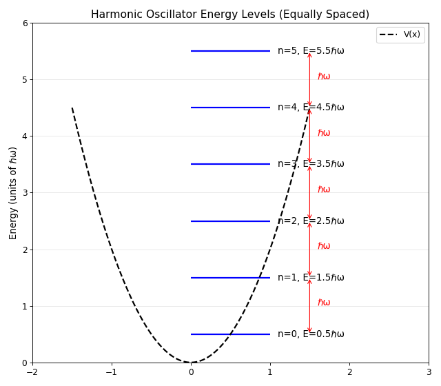
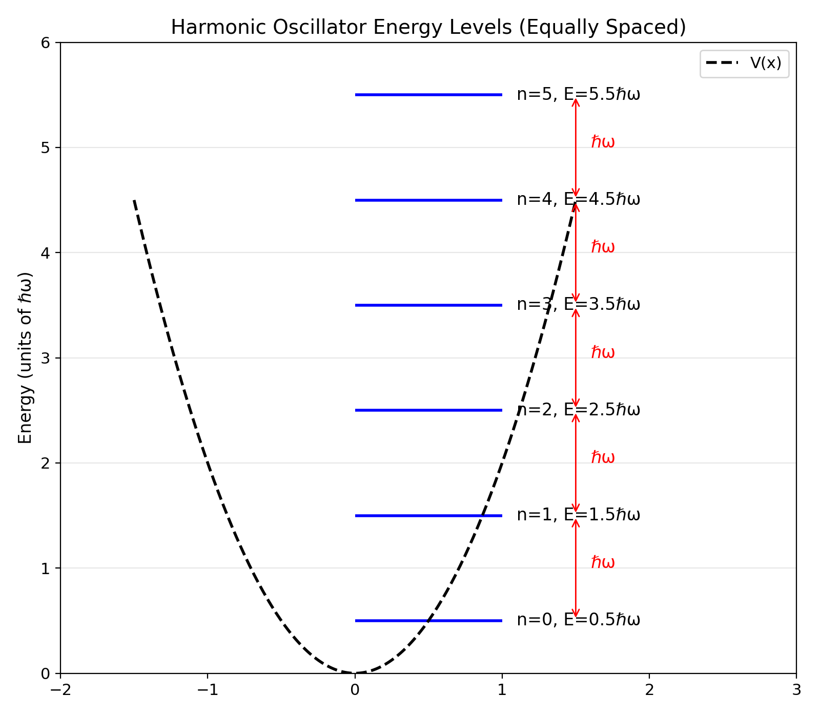
Energy level diagram

(Source code, png, hires.png, pdf)

../_images/plot_harmonic_oscillator_energy_levels.png

The energy levels \(E_n = \hbar\omega(n + \frac{1}{2})\) are shown as horizontal blue lines overlaid on the parabolic potential \(V(x) = \frac{1}{2}m\omega^2 x^2\). The red arrows indicate the constant spacing \(\Delta E = \hbar\omega\) between adjacent levels. This equal spacing is a defining feature of the harmonic oscillator and arises from the commutation relation \([\hat{a}, \hat{a}^\dagger] = 1\) of the ladder operators.

Key difference from particle in a box: Energy levels are equally spaced by \(\Delta E = \hbar\omega\), unlike the particle in a box where spacing increases with \(n\).

Classical vs quantum comparison

Classical turning points vs quantum probability

One of the most striking differences between classical and quantum mechanics appears when we compare where particles are most likely to be found.

Classical turning points: For a classical particle with energy \(E\) in potential \(V(x)\), the turning points \(x_{\text{turn}}\) are where the potential equals the total energy:

\[E = V(x_{\text{turn}})\]

For the harmonic oscillator \(V(x) = \frac{1}{2}m\omega^2 x^2\) with energy \(E_n = \hbar\omega(n + \frac{1}{2})\):

\[\hbar\omega\left(n + \frac{1}{2}\right) = \frac{1}{2}m\omega^2 x_{\text{turn}}^2\]

Solving for the turning points:

\[x_{\text{turn}} = \pm\sqrt{\frac{\hbar(2n + 1)}{m\omega}} = \pm\sqrt{\frac{2E_n}{m\omega^2}}\]

Physical meaning: Classically, the particle cannot go beyond these points because it would need \(E > V(x)\), which violates energy conservation. At the turning points, all energy is potential (\(K = 0\)), so the particle momentarily stops before reversing direction.

Where is the particle most likely found?

Classical: Particle spends most time at turning points (where it slows down)

Classical probability density:

\[P_{\text{classical}}(x) \propto \frac{1}{v(x)} \propto \frac{1}{\sqrt{E - V(x)}}\]

Peaks at \(x = \pm A\) (turning points) and minimum at \(x = 0\).

Reason: At the turning points, velocity \(v \to 0\), so the particle spends more time there. At the center (\(x = 0\)), velocity is maximum, so the particle zips through quickly.

Quantum ground state (\(n=0\)): Most probable at \(x = 0\) (center!)

This is opposite to classical prediction! The quantum probability density \(|\psi_0(x)|^2 \propto e^{-m\omega x^2/\hbar}\) is a Gaussian centered at \(x = 0\) with maximum at the center.

Why the difference?

Classical: Particle has definite trajectory, slows at turning points
Quantum: Particle described by spread out wavefunction, no definite trajectory
Ground state wavefunction has simplest form (fewest nodes), concentrated at center

Quantum excited states: For large \(n\), probability distribution approaches classical prediction (correspondence principle).

Comparing quantum and classical for \(n = 10\):

Classical: Two sharp peaks at \(x = \pm\sqrt{21\hbar/(m\omega)}\)
Quantum: Oscillating probability with envelope approaching classical
Average over oscillations matches classical distribution

Comparing quantum and classical for \(n = 0\):

Classical turning points: \(x = \pm\sqrt{\hbar/(m\omega)}\)
Quantum maximum: \(x = 0\)
Quantum probability at turning points: \(|\psi_0(\pm\sqrt{\hbar/(m\omega)})|^2 \approx 0.6 |\psi_0(0)|^2\) (significant but not maximum)

Quantum tunneling into classically forbidden regions

Classical mechanics: Particle cannot exist where \(E < V(x)\). Beyond the turning points, kinetic energy would be negative (\(K = E - V < 0\)), which is impossible.

Quantum mechanics: Wavefunction extends into classically forbidden regions!

For the harmonic oscillator ground state, the probability of finding the particle beyond the classical turning points is:

\[P(|x| > x_{\text{turn}}) = \int_{|x| > \sqrt{\hbar/(m\omega)}} |\psi_0(x)|^2 dx \approx 0.16\]

About 16% of the time, the particle is found where it “shouldn’t” be classically!

Why this happens: The wavefunction is continuous and smooth. It cannot suddenly become zero at the turning points. Instead, it decays exponentially into the classically forbidden region:

\[\psi(x) \propto e^{-\sqrt{2m[V(x) - E]}/\hbar \cdot x} \quad \text{for } x > x_{\text{turn}}\]

Physical consequences:

Quantum tunneling: Particles can penetrate barriers (alpha decay, scanning tunneling microscopy)

Zero point energy required: If wavefunction were zero beyond turning points, kinetic energy would be infinite (discontinuous derivative)

Uncertainty principle: Confining particle more tightly (smaller \(x_{\text{turn}}\)) increases momentum uncertainty

Energy and position relationship

Energy determines accessible region:

For the harmonic oscillator at energy \(E_n\):

Classically allowed: \(|x| \leq \sqrt{2E_n/(m\omega^2)}\)

Most of quantum probability within: \(|x| \lesssim \sqrt{(2n+1)\hbar/(m\omega)}\)

Wavefunction spreads as \(\Delta x \propto \sqrt{n + 1/2}\)

Higher energy states spread out more:

State

Classical turning points

Quantum uncertainty \(\Delta x\)

\(n=0\)

\(\pm\sqrt{\hbar/(m\omega)}\)

\(\sqrt{\hbar/(2m\omega)}\)

\(n=1\)

\(\pm\sqrt{3\hbar/(m\omega)}\)

\(\sqrt{3\hbar/(2m\omega)}\)

\(n=10\)

\(\pm\sqrt{21\hbar/(m\omega)}\)

\(\sqrt{21\hbar/(2m\omega)}\)

Notice: \(\Delta x \approx x_{\text{turn}}/\sqrt{2}\) for all states (quantum uncertainty comparable to classical amplitude).

Correspondence principle: As \(n \to \infty\), quantum mechanics reproduces classical results. The quantum probability density oscillates rapidly and its average matches the classical distribution.

Coherent states: The most classical quantum states

What are coherent states?

While energy eigenstates \(|n\rangle\) are stationary and have definite energy, they do not behave like classical oscillators. There is another type of quantum state that exhibits the most classical like behavior possible in quantum mechanics: coherent states.

A coherent state \(|\alpha\rangle\) is defined as an eigenstate of the annihilation operator:

\[\hat{a}|\alpha\rangle = \alpha |\alpha\rangle\]

where \(\alpha\) is a complex number (not a quantum number like \(n\)).

Key difference from energy eigenstates:

Energy eigenstates: \(\hat{H}|n\rangle = E_n|n\rangle\) (Hermitian operator, real eigenvalues)
Coherent states: \(\hat{a}|\alpha\rangle = \alpha|\alpha\rangle\) (non-Hermitian operator, complex eigenvalues)

Why are coherent states important?

Coherent states are special because they:

Minimize the uncertainty principle: \(\Delta x \cdot \Delta p = \hbar/2\) (saturate the bound, like the ground state)
Maintain their shape over time: They remain coherent states but with oscillating phase
Most closely resemble classical oscillation: The expectation values \(\langle x(t) \rangle\) and \(\langle p(t) \rangle\) follow classical trajectories
Describe laser light: Photons in a laser beam are in coherent states
Form an overcomplete basis: Any state can be expanded in coherent states (though they’re not orthogonal)

Constructing coherent states from energy eigenstates

A coherent state can be written as a superposition of energy eigenstates:

\[|\alpha\rangle = e^{-|\alpha|^2/2} \sum_{n=0}^{\infty} \frac{\alpha^n}{\sqrt{n!}} |n\rangle\]

Why this form? Let’s verify it satisfies \(\hat{a}|\alpha\rangle = \alpha|\alpha\rangle\).

Proving the eigenvalue equation

Apply \(\hat{a}\) to the coherent state:

\[\hat{a}|\alpha\rangle = e^{-|\alpha|^2/2} \sum_{n=0}^{\infty} \frac{\alpha^n}{\sqrt{n!}} \hat{a}|n\rangle\]

Use \(\hat{a}|n\rangle = \sqrt{n}|n-1\rangle\):

\[= e^{-|\alpha|^2/2} \sum_{n=0}^{\infty} \frac{\alpha^n}{\sqrt{n!}} \sqrt{n}|n-1\rangle\]

\[= e^{-|\alpha|^2/2} \sum_{n=1}^{\infty} \frac{\alpha^n \sqrt{n}}{\sqrt{n!}} |n-1\rangle\]

Change summation index: let \(m = n-1\), so \(n = m+1\):

\[= e^{-|\alpha|^2/2} \sum_{m=0}^{\infty} \frac{\alpha^{m+1} \sqrt{m+1}}{\sqrt{(m+1)!}} |m\rangle\]

Simplify: \(\sqrt{m+1}/\sqrt{(m+1)!} = \sqrt{m+1}/[\sqrt{m+1}\sqrt{m!}] = 1/\sqrt{m!}\):

\[= e^{-|\alpha|^2/2} \sum_{m=0}^{\infty} \frac{\alpha^{m+1}}{\sqrt{m!}} |m\rangle\]

\[= \alpha \cdot e^{-|\alpha|^2/2} \sum_{m=0}^{\infty} \frac{\alpha^{m}}{\sqrt{m!}} |m\rangle\]

\[= \alpha |\alpha\rangle \quad \checkmark\]

This proves \(\hat{a}|\alpha\rangle = \alpha|\alpha\rangle\).

Alternative construction: Displacement operator

Coherent states can also be generated by applying the displacement operator to the ground state:

\[|\alpha\rangle = \hat{D}(\alpha)|0\rangle\]

where the displacement operator is:

\[\hat{D}(\alpha) = e^{\alpha \hat{a}^\dagger - \alpha^* \hat{a}}\]

Physical interpretation: \(\hat{D}(\alpha)\) shifts the ground state wavefunction in phase space by an amount determined by \(\alpha\). This “displaces” the Gaussian wavepacket from the origin without changing its shape.

Time evolution of coherent states

Key property: Coherent states remain coherent states as they evolve!

At time \(t\), the coherent state becomes:

\[|\alpha(t)\rangle = |\alpha e^{-i\omega t}\rangle\]

The parameter \(\alpha\) simply picks up a rotating phase factor \(e^{-i\omega t}\).

Expectation values oscillate classically:

\[\langle x(t) \rangle = \sqrt{\frac{2\hbar}{m\omega}} |\alpha| \cos(\omega t + \phi)\]

\[\langle p(t) \rangle = -\sqrt{2m\hbar\omega} |\alpha| \sin(\omega t + \phi)\]

where \(\phi = \arg(\alpha)\) is the phase of \(\alpha\).

Physical meaning: The expectation values trace out an ellipse in phase space with angular frequency \(\omega\), exactly like a classical harmonic oscillator!

Uncertainty in coherent states

For any coherent state \(|\alpha\rangle\):

\[\Delta x = \sqrt{\frac{\hbar}{2m\omega}}, \quad \Delta p = \sqrt{\frac{m\hbar\omega}{2}}\]

\[\Delta x \cdot \Delta p = \frac{\hbar}{2}\]

Key observations:

The uncertainties are independent of \(\alpha\) (same as ground state!)

The uncertainty product achieves the minimum \(\hbar/2\)

Unlike energy eigenstates \(|n\rangle\) where \(\Delta x\) grows with \(\sqrt{n}\), coherent states maintain constant spread

Physical picture: Coherent states are Gaussian wavepackets that oscillate back and forth without changing shape or spreading. This is the most “particle like” behavior possible in quantum mechanics.

Coherent states vs energy eigenstates

Property

Energy eigenstates \(|n\rangle\)

Coherent states \(|\alpha\rangle\)

Eigenvalue equation

\(\hat{H}|n\rangle = E_n|n\rangle\)

\(\hat{a}|\alpha\rangle = \alpha|\alpha\rangle\)

Eigenvalue type

Real (\(E_n\))

Complex (\(\alpha\))

Energy

Definite (\(E_n\))

Uncertain (Poisson distribution)

Time evolution

Phase rotation only

Oscillation in phase space

\(\langle x \rangle, \langle p \rangle\)

Both zero

Oscillate like classical particle

Uncertainty \(\Delta x \cdot \Delta p\)

\(\hbar(n + \frac{1}{2}) \geq \frac{\hbar}{2}\)

\(\frac{\hbar}{2}\) (minimum)

Classical behavior

Stationary, spread out

Localized, oscillating

Physical example

Definite energy quantum state

Laser light, classical limit

Why coherent states matter in physics

1. Quantum optics: Coherent states describe the quantum state of laser light. A laser produces photons in a coherent state, which is why laser light is so different from thermal light.

2. Classical limit: Coherent states with large \(|\alpha|\) behave most like classical oscillators. As \(|\alpha| \to \infty\), quantum mechanics → classical mechanics.

3. Quantum communication: Coherent states are used in quantum key distribution protocols because they can be generated and detected efficiently.

4. Squeezed states: Generalizations of coherent states where \(\Delta x\) and \(\Delta p\) can be different (but still \(\Delta x \cdot \Delta p \geq \hbar/2\)). These are used in gravitational wave detectors to improve sensitivity.

5. Path integral formulation: Coherent states provide a natural connection between quantum mechanics and classical mechanics in the path integral approach.

The measurement problem for coherent states

If you measure the energy of a coherent state \(|\alpha\rangle\), you get different values \(E_n\) with probabilities:

\[P(n) = |\langle n | \alpha \rangle|^2 = e^{-|\alpha|^2} \frac{|\alpha|^{2n}}{n!}\]

This is a Poisson distribution with mean \(\langle n \rangle = |\alpha|^2\).

Physical interpretation: Even though \(\langle x(t) \rangle\) and \(\langle p(t) \rangle\) behave classically, the energy is uncertain! A coherent state is a superposition of many energy eigenstates. This is fundamentally different from classical physics, where a definite trajectory implies definite energy.

Key insight: Different bases for different purposes

Quantum mechanics allows us to expand any state in different bases:

Energy eigenstates \(|n\rangle\): Natural for stationary problems, time independent Hamiltonians

Coherent states \(|\alpha\rangle\): Natural for dynamics, classical correspondence, quantum optics

Position eigenstates \(|x\rangle\): Natural for position measurements

Momentum eigenstates \(|p\rangle\): Natural for momentum measurements

The physics is the same regardless of which basis you choose, but some calculations are easier in certain bases!

Key insights and gotchas

Important takeaways from the harmonic oscillator

The quantum harmonic oscillator teaches several profound lessons that generalize to all of quantum mechanics:

1. Zero-point energy is unavoidable

The ground state energy \(E_0 = \frac{1}{2}\hbar\omega \neq 0\) is not due to thermal fluctuations—it exists even at absolute zero temperature!

Why it exists:

Required by Heisenberg uncertainty principle: \(\Delta x \cdot \Delta p \geq \hbar/2\)
If \(E = 0\), both position and momentum would be exactly zero (violates uncertainty)
The particle must have some “wiggle room” to satisfy quantum mechanics

Physical consequences:

Helium remains liquid at absolute zero (zero-point motion prevents crystallization)
Casimir effect: vacuum energy between conducting plates
Limits of measurement precision at quantum scales

2. Operators don’t commute—order matters!

Critical gotcha: \(\hat{a}\hat{a}^\dagger \neq \hat{a}^\dagger\hat{a}\)!

\[\hat{a}\hat{a}^\dagger = \hat{a}^\dagger\hat{a} + 1\]

This is not a small correction—it’s the entire \(\frac{1}{2}\hbar\omega\) zero-point energy!

Why order matters: Operators are operations (measurements), and the order you perform measurements affects the result. Position then momentum ≠ momentum then position.

3. The commutator encodes everything

The single relation \([\hat{a}, \hat{a}^\dagger] = 1\) completely determines:

Energy spectrum (equally spaced levels)
Spacing between levels (\(\hbar\omega\))
State structure (ladder of excited states)
Transition rules (selection rules)

Deep insight: Quantum mechanics is fundamentally about commutation relations, not differential equations!

4. Classical limit requires large quantum numbers

Common misconception: “Higher energy = more quantum”

Reality: Higher energy = more classical!

For large \(n\):

Energy levels become continuous (spacing \(\hbar\omega\) becomes negligible compared to \(E_n\))
Probability distribution approaches classical prediction
Relative uncertainty decreases: \(\Delta E/E \sim 1/n \to 0\)

This is the correspondence principle: quantum mechanics → classical mechanics as quantum numbers become large.

5. Equal spacing is special

Why it matters: The harmonic oscillator is the only potential with equally-spaced energy levels!

Consequence: Any system with equally-spaced levels must be approximately harmonic near equilibrium.

Applications:

Molecular vibrations (bonds are approximately harmonic springs)
Phonons in solids (lattice vibrations)
Photons in cavities (electromagnetic modes)

Gotcha: Real molecules deviate from harmonic behavior at high energies (anharmonicity) and can dissociate.

6. Ladder operators are more than a trick

Not just a mathematical convenience: Creation and annihilation operators reveal the particle nature of excitations.

Physical meaning:

\(\hat{a}^\dagger\) creates a quantum of energy \(\hbar\omega\) (particle interpretation)
\(\hat{a}\) destroys a quantum
\(\hat{N} = \hat{a}^\dagger\hat{a}\) counts the number of quanta

Foundation of modern physics:

Quantum field theory: particles are quanta of fields
Photons: quanta of electromagnetic field
Phonons: quanta of vibrations
All particles in nature are field excitations

7. Ground state is never “at rest”

Common misconception: \(n=0\) means the particle is stationary at the bottom of the potential.

Reality: The ground state has maximum probability at \(x=0\), but:

\(\Delta x \neq 0\) (position uncertainty)
\(\Delta p \neq 0\) (momentum uncertainty)
Kinetic energy \(\langle T \rangle = \frac{1}{4}\hbar\omega\)
Potential energy \(\langle V \rangle = \frac{1}{4}\hbar\omega\)
Total: \(E_0 = \frac{1}{2}\hbar\omega\)

The particle is always in motion at the quantum level!

8. Energy eigenstates are stationary

Key property: If the system is in state \(|n\rangle\), it stays in that state forever (for time-independent Hamiltonian).

\[|\psi_n(x,t)|^2 = |\psi_n(x)|^2 e^{-iE_n t/\hbar} e^{+iE_n t/\hbar} = |\psi_n(x)|^2\]

The phase oscillates, but probability density is constant!

Gotcha: Real systems are usually in superpositions, which do evolve in time and show interference effects.

9. The uncertainty principle appears naturally

The ground state wavefunction \(\psi_0(x) \propto e^{-m\omega x^2/(2\hbar)}\) is a Gaussian.

For a Gaussian, the product \(\Delta x \cdot \Delta p\) achieves the minimum value allowed by Heisenberg:

\[\Delta x \cdot \Delta p = \frac{\hbar}{2}\]

Deep fact: The ground state is the most localized state possible in quantum mechanics—it minimizes uncertainty!

Higher excited states have \(\Delta x \cdot \Delta p > \hbar/2\) (more uncertainty).

10. Selection rules from symmetry

The harmonic oscillator potential is symmetric: \(V(-x) = V(x)\).

Consequence: Wavefunctions have definite parity:

Even \(n\): \(\psi_n(-x) = +\psi_n(x)\) (symmetric)
Odd \(n\): \(\psi_n(-x) = -\psi_n(x)\) (antisymmetric)

Selection rule for electric dipole transitions: \(\Delta n = \pm 1\) only!

Cannot go from \(n=0\) to \(n=2\) directly by absorbing a single photon (requires \(\Delta n = \pm 1, \pm 3, \pm 5, \ldots\)).

Common mistakes to avoid

Mistake 1: Forgetting the zero-point energy

Wrong: “Ground state means \(E = 0\)”

Right: Ground state has \(E_0 = \frac{1}{2}\hbar\omega\)

Mistake 2: Treating operators like numbers

Wrong: \(\hat{x}\hat{p} = \hat{p}\hat{x}\)

Right: \([\hat{x}, \hat{p}] = i\hbar\), so \(\hat{x}\hat{p} = \hat{p}\hat{x} + i\hbar\)

Mistake 3: Confusing energy eigenstates with time evolution

Wrong: “The system is in \(|n\rangle\), so it’s not changing”

Right: Energy eigenstates are stationary, but superpositions evolve! Most real states are superpositions.

Mistake 4: Thinking quantum = small

Wrong: “Quantum effects only matter at atomic scales”

Right: Quantum effects matter when \(\hbar\omega\) is comparable to thermal energy \(kT\) or measurement resolution. Macroscopic quantum phenomena exist (superconductivity, superfluidity, quantum Hall effect).

Mistake 5: Expecting classical behavior at low energy

Wrong: “Low energy means classical behavior”

Right: Ground state (\(n=0\)) is the most quantum! Classical behavior emerges at high quantum numbers (correspondence principle).

Mistake 6: Forgetting normalization matters

Wrong: \(|n\rangle = (\hat{a}^\dagger)^n |0\rangle\)

Right: \(|n\rangle = \frac{1}{\sqrt{n!}} (\hat{a}^\dagger)^n |0\rangle\)

The \(\sqrt{n!}\) is essential for proper normalization!

Why the harmonic oscillator is everywhere

The harmonic oscillator is the most important problem in physics. Here’s why:

1. Taylor expansion near equilibrium

Any smooth potential near a minimum can be approximated as:

\[V(x) \approx V(x_0) + \underbrace{V'(x_0)}_{=0 \text{ at minimum}} (x-x_0) + \frac{1}{2}V''(x_0)(x-x_0)^2 + \ldots\]

\[V(x) \approx V_0 + \frac{1}{2}k(x-x_0)^2 \quad \text{where } k = V''(x_0)\]

This is a harmonic oscillator!

Examples:

Atoms in molecules (bonds stretch/compress)
Atoms in solids (vibrate around lattice sites)
Electrons in atoms (small oscillations around equilibrium)

2. Normal modes decompose into independent oscillators

Any coupled system of oscillators can be transformed into independent harmonic oscillators using normal mode analysis.

Examples:

Molecular vibrations (3N-6 vibrational modes for N atoms)
Phonons in solids (lattice vibrations)
String vibrations (musical instruments)

3. Quantum field theory foundation

In quantum field theory:

Fields are decomposed into Fourier modes
Each mode is a harmonic oscillator
Particles are quanta of these oscillators!

All particles (photons, electrons, quarks, etc.) are described this way.

Perturbation theory

Why do we need perturbation theory?

We have seen that most quantum systems cannot be solved exactly. We can solve:

Particle in a box ✓
Harmonic oscillator ✓
Hydrogen atom ✓

However, we cannot solve exactly:

Helium atom (3-body problem with electron-electron repulsion)
Hydrogen atom in external fields
Anharmonic oscillators
Most real molecules and solids

Here, perturbation theory gives us a systematic way to find approximate solutions when the Hamiltonian is “close” to a solvable problem!

The basic idea

Splitting the Hamiltonian

We suppose that we can write:

\[\hat{H} = \hat{H}_0 + \hat{H}'\]

Here, we have:

\(\hat{H}_0\): Exactly solvable (we know eigenstates \(|n^{(0)}\rangle\) and energies \(E_n^{(0)}\))
\(\hat{H}'\): Small perturbation (we cannot solve, but it’s “small”)

Goal: We want to find the perturbed energies \(E_n\) and states \(|n\rangle\) of the full Hamiltonian \(\hat{H}\).

What does “small” mean?

We say the perturbation is small if its matrix elements are much less than the energy gaps:

\[|\langle m^{(0)} | \hat{H}' | n^{(0)} \rangle| \ll |E_m^{(0)} - E_n^{(0)}|\]

Example: For hydrogen atom in a weak electric field, we require that the field-induced energy shifts should be much smaller than the spacing between energy levels.

Time-independent perturbation theory

The perturbation expansion

We introduce a bookkeeping parameter \(\lambda\) (we will set it to 1 at the end):

\[\hat{H} = \hat{H}_0 + \lambda\hat{H}'\]

We then expand energies and states in powers of \(\lambda\):

\[E_n = E_n^{(0)} + \lambda E_n^{(1)} + \lambda^2 E_n^{(2)} + \cdots\]

\[|n\rangle = |n^{(0)}\rangle + \lambda|n^{(1)}\rangle + \lambda^2|n^{(2)}\rangle + \cdots\]

Here, we have indicated with the superscripts the order of perturbation theory.

Non-degenerate perturbation theory

First-order energy correction

We find that to first order in \(\lambda\), the energy shift is:

\[\boxed{E_n^{(1)} = \langle n^{(0)} | \hat{H}' | n^{(0)} \rangle}\]

Physical interpretation: We see that this is simply the expectation value of the perturbation in the unperturbed state.

Example: Ground state energy of hydrogen in a uniform electric field \(\mathcal{E}\):

Perturbation: \(\hat{H}' = e\mathcal{E} z\)
By symmetry: \(\langle 1s | z | 1s \rangle = 0\)
Therefore: \(E_1^{(1)} = 0\) (we see there is no first-order shift!)

First-order wavefunction correction

We obtain the first-order correction to the wavefunction as:

\[\boxed{|n^{(1)}\rangle = \sum_{m \neq n} \frac{\langle m^{(0)} | \hat{H}' | n^{(0)} \rangle}{E_n^{(0)} - E_m^{(0)}} |m^{(0)}\rangle}\]

Key insight: We see that the perturbation “mixes in” other states, with weights inversely proportional to the energy difference.

Note: We observe that states with \(E_m^{(0)} \approx E_n^{(0)}\) contribute strongly (this is why near-degeneracies are problematic!).

Second-order energy correction

We find that the second-order energy shift is:

\[\boxed{E_n^{(2)} = \sum_{m \neq n} \frac{|\langle m^{(0)} | \hat{H}' | n^{(0)} \rangle|^2}{E_n^{(0)} - E_m^{(0)}}}\]

Important observations:

We see that this always involves a sum over all other states (this can be difficult to compute!)
We notice that the sign depends on whether \(E_m^{(0)} > E_n^{(0)}\) or \(E_m^{(0)} < E_n^{(0)}\):
- Higher states (\(m > n\)) lower the energy (\(E_n^{(2)} < 0\))
- Lower states (\(m < n\)) raise the energy (\(E_n^{(2)} > 0\))
For the ground state, we have all \(m > 0\), so:

\[E_0^{(2)} = \sum_{m > 0} \frac{|\langle m^{(0)} | \hat{H}' | 0^{(0)} \rangle|^2}{E_0^{(0)} - E_m^{(0)}} < 0\]

We see that the ground state energy always decreases to second order!

Example: Anharmonic oscillator

The problem

Let us consider a harmonic oscillator with a small cubic perturbation:

\[\hat{H} = \frac{\hat{p}^2}{2m} + \frac{1}{2}m\omega^2\hat{x}^2 + \lambda\hat{x}^3\]

We know \(\hat{H}_0\) exactly. What is the effect of \(\hat{H}' = \lambda\hat{x}^3\)?

First-order energy correction

We calculate:

\[E_n^{(1)} = \langle n | \hat{x}^3 | n \rangle = 0\]

Why zero? We see that \(\hat{x}^3\) is an odd function, and \(|n\rangle\) has definite parity:

\[\langle n | \hat{x}^3 | n \rangle = -\langle n | \hat{x}^3 | n \rangle = 0\]

So we find that the first-order shift vanishes by symmetry!

Second-order energy correction

Here, we need matrix elements \(\langle m | \hat{x}^3 | n \rangle\). Using ladder operators:

\[\hat{x} = \sqrt{\frac{\hbar}{2m\omega}}(\hat{a} + \hat{a}^\dagger)\]

\[\hat{x}^3 = \left(\frac{\hbar}{2m\omega}\right)^{3/2} (\hat{a} + \hat{a}^\dagger)^3\]

We see that this connects \(|n\rangle\) to \(|n \pm 1\rangle\) and \(|n \pm 3\rangle\). The calculation gives:

\[E_n^{(2)} = -\frac{15\lambda^2\hbar}{4m^3\omega^5}(n^2 + n + \frac{11}{30})\]

We observe that the energy decreases for all states, as we expect for ground state and consistent with our general result.

Degenerate perturbation theory

The problem with degeneracy

If we have \(E_m^{(0)} = E_n^{(0)}\) for \(m \neq n\), then:

\[|n^{(1)}\rangle \propto \frac{1}{E_n^{(0)} - E_m^{(0)}} \to \infty\]

We see that the formulas blow up! We need a different approach.

The solution: Diagonalize in degenerate subspace

Procedure:

We identify the degenerate subspace (dimension \(d\))
We form the \(d \times d\) matrix of \(\hat{H}'\) within this subspace:

\[W_{ij} = \langle i^{(0)} | \hat{H}' | j^{(0)} \rangle \quad (i, j = 1, \ldots, d)\]

We diagonalize this matrix to find eigenvalues \(E_i^{(1)}\) and eigenvectors
We see that the eigenvectors give the “correct” zeroth-order states that diagonalize \(\hat{H}'\)
We then use non-degenerate perturbation theory for higher orders

Example: Stark effect in hydrogen

Hydrogen in a uniform electric field

Let us apply an electric field \(\vec{\mathcal{E}} = \mathcal{E}\hat{z}\) to a hydrogen atom:

\[\hat{H}' = e\mathcal{E}z = e\mathcal{E}r\cos\theta\]

Question: What happens to the \(n=2\) level (which has \(l=0\) and \(l=1\) states)?

The \(n=2\) level

We have four states: \(|2s\rangle\), \(|2p, m=0\rangle\), \(|2p, m=\pm 1\rangle\)

All have the same energy \(E_2^{(0)} = -13.6 \text{ eV}/4 = -3.4\) eV (degenerate!).

Selection rules save us

We see that the perturbation \(\hat{H}' \propto z = r\cos\theta\) changes \(l\) by 1 (dipole selection rule):

\[\langle 2s | z | 2p, m=0 \rangle \neq 0\]

But:

\[\langle 2s | z | 2s \rangle = 0, \quad \langle 2p | z | 2p \rangle = 0, \quad \langle 2s | z | 2p, m=\pm 1 \rangle = 0\]

So we only need to consider the \(2 \times 2\) subspace of \(\{|2s\rangle, |2p, m=0\rangle\}\).

Diagonalizing the perturbation

We form the matrix:

\[\begin{split}W = \begin{pmatrix} 0 & \langle 2s | e\mathcal{E}z | 2p_0 \rangle \\ \langle 2p_0 | e\mathcal{E}z | 2s \rangle & 0 \end{pmatrix} = \begin{pmatrix} 0 & -3ea_0\mathcal{E} \\ -3ea_0\mathcal{E} & 0 \end{pmatrix}\end{split}\]

We find the eigenvalues:

\[E_\pm^{(1)} = \pm 3ea_0\mathcal{E}\]

We see that the degeneracy is lifted! The \(n=2\) level splits into two by the electric field (linear Stark effect).

import numpy as np
import matplotlib.pyplot as plt

fig, ax = plt.subplots(figsize=(12, 8))

# Energy levels
E2 = -3.4  # eV

# No field (left)
x_left = 1
ax.plot([x_left-0.3, x_left+0.3], [E2, E2], color='#2E86AB', linewidth=4, label='n=2 (4-fold degenerate)')
ax.text(x_left-0.5, E2, '$n=2$', fontsize=26, weight='bold', ha='right', va='center')
ax.text(x_left+0.5, E2+0.1, '2s, 2p$_{0,\pm 1}$\n(4 states)', fontsize=22, ha='left', va='bottom')

# With field (right)
x_right = 3
splitting = 0.6
ax.plot([x_right-0.3, x_right+0.3], [E2 + splitting, E2 + splitting], color='#C73E1D', linewidth=4)
ax.plot([x_right-0.3, x_right+0.3], [E2 - splitting, E2 - splitting], color='#6A994E', linewidth=4)
ax.plot([x_right-0.3, x_right+0.3], [E2, E2], color='#A23B72', linewidth=4, alpha=0.7)

# Labels for split levels
ax.text(x_right+0.5, E2 + splitting, '$E_+ = E_2 + 3ea_0\mathcal{E}$', fontsize=22, ha='left', va='center')
ax.text(x_right+0.5, E2 - splitting, '$E_- = E_2 - 3ea_0\mathcal{E}$', fontsize=22, ha='left', va='center')
ax.text(x_right+0.5, E2, '2p$_{\pm 1}$ (unchanged)', fontsize=22, ha='left', va='center', style='italic')

# Arrows showing splitting
ax.annotate('', xy=(x_right, E2 + splitting), xytext=(x_right, E2),
           arrowprops=dict(arrowstyle='<->', lw=2, color='#C73E1D'))
ax.annotate('', xy=(x_right, E2), xytext=(x_right, E2 - splitting),
           arrowprops=dict(arrowstyle='<->', lw=2, color='#6A994E'))

# Transition arrow
ax.annotate('', xy=(x_right-0.5, E2), xytext=(x_left+0.5, E2),
           arrowprops=dict(arrowstyle='->', lw=3, color='#2E86AB', linestyle='--'))
ax.text(2, E2+0.8, 'Apply field $\mathcal{E}$', fontsize=24, ha='center', weight='bold', color='#2E86AB')

# Formatting
ax.set_xlim([0, 5])
ax.set_ylim([-4.5, -2.5])
ax.set_ylabel('Energy (eV)', fontsize=28, weight='bold')
ax.set_title('Linear Stark effect in hydrogen (n=2 level)', fontsize=28, weight='bold')
ax.set_xticks([x_left, x_right])
ax.set_xticklabels(['$\mathcal{E} = 0$', '$\mathcal{E} \\neq 0$'], fontsize=26)
ax.tick_params(axis='y', labelsize=24)
ax.grid(axis='y', alpha=0.3)
ax.spines['top'].set_visible(False)
ax.spines['right'].set_visible(False)

plt.tight_layout()

(Source code, png, hires.png, pdf)

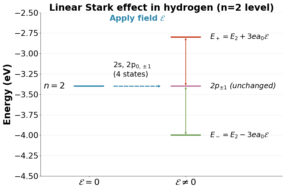
Time-dependent perturbation theory

The time-dependent problem

Let us now suppose that the perturbation varies with time:

\[\hat{H}(t) = \hat{H}_0 + \hat{H}'(t)\]

Question: If the system starts in state \(|i\rangle\) at \(t=0\), what is the probability to find it in state \(|f\rangle\) at time \(t\)?

This is crucial for:

Absorption and emission of radiation
Scattering processes
Decay rates and lifetimes

First-order transition probability

We find that the probability of transitioning from \(|i\rangle\) to \(|f\rangle\) (with \(f \neq i\)) is:

\[P_{i \to f}(t) = \frac{1}{\hbar^2}\left|\int_0^t \langle f | \hat{H}'(t') | i \rangle e^{i\omega_{fi}t'} dt'\right|^2\]

Here, we have defined \(\omega_{fi} = (E_f - E_i)/\hbar\) as the transition frequency.

Harmonic perturbation

For a sinusoidal perturbation (e.g., electromagnetic wave):

\[\hat{H}'(t) = \hat{V}\cos(\omega t) = \frac{\hat{V}}{2}(e^{i\omega t} + e^{-i\omega t})\]

We evaluate the integral and obtain:

\[P_{i \to f}(t) = \frac{|\langle f | \hat{V} | i \rangle|^2}{\hbar^2} \frac{\sin^2[(\omega_{fi} - \omega)t/2]}{(\omega_{fi} - \omega)^2}\]

Resonance condition

We see that the transition probability is largest when \(\omega \approx \omega_{fi}\):

\[\hbar\omega = E_f - E_i\]

This is the Bohr frequency condition! We observe that resonance occurs when the photon energy matches the energy gap.

At resonance, we find that \(P_{i \to f}(t) \propto t^2\) (it grows quadratically for short times).

Fermi’s golden rule

Transition to a continuum

Often, we have that the final state is part of a continuum (e.g., photoionization, particle decay). We sum over many final states with density \(\rho(E_f)\):

\[\Gamma_{i \to f} = \sum_f P_{i \to f}(t)/t \to \int dE_f \, \rho(E_f) \, P_{i \to f}(t)/t\]

Fermi’s golden rule

Taking the limit \(t \to \infty\) and using the identity:

\[\lim_{t \to \infty} \frac{\sin^2[(\omega_{fi} - \omega)t/2]}{(\omega_{fi} - \omega)^2} = \frac{\pi t}{2}\delta(\omega_{fi} - \omega)\]

We obtain:

\[\boxed{\Gamma_{i \to f} = \frac{2\pi}{\hbar}|\langle f | \hat{H}' | i \rangle|^2 \rho(E_f)}\]

This is Fermi’s golden rule – one of the most important formulas in quantum mechanics!

Interpretation:

\(\Gamma\): Transition rate (probability per unit time)
We see it is proportional to \(|\langle f | \hat{H}' | i \rangle|^2\): Matrix element squared
We also see it is proportional to \(\rho(E_f)\): Density of final states (more available states means faster transition)

Applications of Fermi’s golden rule

1. Spontaneous emission: Atom decays from excited state to ground state, emitting a photon

\[\Gamma = \frac{\omega^3}{3\pi\epsilon_0\hbar c^3}|\langle f | \vec{d} | i \rangle|^2\]

Here, we have \(\vec{d} = -e\vec{r}\) as the dipole moment.

2. Photoionization: Photon ionizes an atom (electron ejected to continuum)

3. Beta decay: Neutron decays to proton + electron + antineutrino

4. Scattering cross sections: Probability for particle collisions

Example: Hydrogen 2p to 1s transition

The decay rate

We consider an electron in the \(2p\) state that can decay to \(1s\) by emitting a photon.

Using Fermi’s golden rule with the dipole operator:

\[\Gamma_{2p \to 1s} = \frac{\omega^3}{3\pi\epsilon_0\hbar c^3}|\langle 1s | e\vec{r} | 2p \rangle|^2\]

For the \(2p \to 1s\) transition:

Energy: \(\Delta E = 10.2\) eV → \(\omega = 1.55 \times 10^{16}\) rad/s
Dipole moment: \(|\langle 1s | er | 2p \rangle| \approx ea_0\)

We calculate:

\[\Gamma \approx 6.3 \times 10^8 \text{ s}^{-1} \quad \Rightarrow \quad \tau = \frac{1}{\Gamma} \approx 1.6 \text{ ns}\]

We see that the 2p state has a lifetime of about 1.6 nanoseconds! This matches experimental observations.

Selection rules from matrix elements

We find that the matrix element \(\langle f | \vec{r} | i \rangle\) vanishes unless:

\[\Delta l = \pm 1, \quad \Delta m = 0, \pm 1\]

These are the selection rules! We see that they come from angular momentum conservation (photon has spin 1).

Summary: Perturbation theory

Type	Key formula
First-order energy (non-degenerate)	\(E_n^{(1)} = \langle n^{(0)} \| \hat{H}' \| n^{(0)} \rangle\)
Second-order energy	\(E_n^{(2)} = \sum_{m \neq n} \frac{\|\langle m^{(0)} \| \hat{H}' \| n^{(0)} \rangle\|^2}{E_n^{(0)} - E_m^{(0)}}\)
Ground state (2nd order)	Always decreases: \(E_0^{(2)} < 0\)
Degenerate case	Diagonalize \(W_{ij} = \langle i \| \hat{H}' \| j \rangle\) in degenerate subspace
Time-dependent transition	\(P_{i \to f} \propto \|\langle f \| \hat{H}' \| i \rangle\|^2 \frac{\sin^2(\omega t/2)}{\omega^2}\)
Fermi’s golden rule	\(\Gamma = \frac{2\pi}{\hbar}\|\langle f \| \hat{H}' \| i \rangle\|^2 \rho(E_f)\)
Resonance condition	\(\hbar\omega = E_f - E_i\) (Bohr frequency)
Spontaneous emission rate	\(\Gamma \propto \omega^3 \|\langle f \| \vec{d} \| i \rangle\|^2\)

Why perturbation theory matters: We have seen that most real quantum systems cannot be solved exactly. Here, perturbation theory gives us systematic approximations that work remarkably well when the perturbation is small. We see that it explains atomic spectra, chemical bonding, semiconductor physics, and countless other phenomena!

Relativistic quantum mechanics

Schrödinger vs Dirac equation

When do we need the Dirac equation?

The Schrödinger equation is non-relativistic. It works when \(v \ll c\), or equivalently when kinetic energy \(K \ll m_0 c^2\).

The Dirac equation is the relativistic generalization. It’s needed when:

Particle energy approaches rest mass energy (e.g., 511 keV for electrons)
Spin-orbit coupling becomes important
Creating particle-antiparticle pairs is possible

What are relativistic corrections?

For moderate energies (between non-relativistic and fully relativistic), we can use the Schrödinger equation with relativistic corrections:

Relativistic mass: \(m = \gamma m_0\) where \(\gamma = 1/\sqrt{1 - v^2/c^2}\)
Relativistic momentum: \(p = \gamma m_0 v\)
Relativistic wavelength: \(\lambda = h/p\) with relativistic \(p\)
Relativistic energy: \(E = \gamma m_0 c^2 = K + m_0 c^2\)

This is sometimes called the semi-relativistic approximation.

Summary

Key equations

The essential quantum mechanical relations:

de Broglie relation: \(\lambda = h/p\)
Time-dependent Schrödinger equation: \(i\hbar \frac{\partial \psi}{\partial t} = \hat{H} \psi\)
Time-independent Schrödinger equation: \(-\frac{\hbar^2}{2m} \nabla^2 \psi + V(\mathbf{r}) \psi = E \psi\)
Momentum operator: \(\hat{\mathbf{p}} = -i\hbar \nabla\)
Energy-momentum relation: \(E = \frac{p^2}{2m}\) (non-relativistic), \(E^2 = (pc)^2 + (m_0 c^2)^2\) (relativistic)

Conceptual framework

Note

Core principles of quantum mechanics:

Particles are described by wavefunctions \(\psi(\mathbf{r}, t)\) encoding probabilities
Wavefunctions satisfy the Schrödinger equation
Observables become operators (position → multiplication, momentum → derivative)
Only certain quantized energy levels are allowed for bound states
Wave-particle duality: \(\lambda = h/p\) connects particle and wave pictures