SSB (direct ptychogrpahy)
High-level overview
Single sideband (SSB) imaging extracts phase information from 4D-STEM data through a direct, non-iterative process. Here’s how it works in four steps:
1. Collect 4D-STEM data
Scan a focused electron probe across your sample in a grid pattern. At each scan position, record a full 2D diffraction pattern on the detector. This creates a 4D dataset \(I(\mathbf{k}; \mathbf{R})\) where \(\mathbf{R}\) is the scan position and \(\mathbf{k}\) is the detector coordinate.
2. Separate sidebands in Fourier space
Fourier transform over all scan positions: \(G(\mathbf{k}, \mathbf{Q}) = \mathcal{F}_{\mathbf{R} \to \mathbf{Q}}[I(\mathbf{k}; \mathbf{R})]\). This separates the signal into three components:
Center disk at \(\mathbf{Q} = 0\) (no phase information)
Right sideband at \(\mathbf{Q} = +\mathbf{k}\) (contains object phase)
Left sideband at \(\mathbf{Q} = -\mathbf{k}\) (conjugate of right sideband)
3. Isolate and divide by probe
Select one sideband using a circular aperture, shift it to the center, then divide by the probe intensity: \(\tilde{O}(\mathbf{k}) = S(\mathbf{k}) / |P(\mathbf{k})|^2\). This removes the probe’s influence and isolates the object’s Fourier transform. The probe \(P(\mathbf{k})\) must be either measured from a vacuum region or constructed from known aberration coefficients.
4. Transform back to get phase
Inverse Fourier transform the isolated sideband back to real space: \(o(\mathbf{r}) = \mathcal{F}_{\mathbf{k} \to \mathbf{r}}^{-1}[\tilde{O}(\mathbf{k})]\). Take the imaginary part to extract the phase map \(\phi(x,y) = \text{Im}[o(\mathbf{r})]\), which represents the projected potential of your sample.
Why it’s fast: All operations are linear (Fourier transforms, multiplication, division). No iterative loops, no optimization, no convergence issues.
Key requirement: Works best for thin samples under the weak-phase approximation where the object transmission is \(O(x,y) \approx 1 + i\phi(x,y)\).
The following sections explain the physics, mathematics, and implementation details behind each of these steps.
Why SSB?
Ptychography is a powerful phase retrieval technique, but it has limitations:
Slow reconstruction: Iterative algorithms (ePIE, rPIE) require hundreds to thousands of iterations, making reconstruction computationally expensive
Initialization dependence: Poor initial guesses for the probe or object can lead to slow convergence or failure
Probe uncertainty: The probe function must be recovered simultaneously with the object, adding complexity
Single sideband (SSB) imaging addresses these challenges by providing:
Fast phase extraction: Direct algebraic reconstruction without iteration
Simple probe measurement from reference samples: With a known reference (vacuum, amorphous film), SSB can quickly measure the probe including aberrations. This measured probe can then be used for unknown samples.
Better initialization for iterative ptychography: SSB gives approximate solutions quickly. Both the object phase φ(x,y) and the measured probe P(k) can initialize ePIE/rPIE, dramatically accelerating convergence compared to random initialization.
SSB is particularly valuable in two scenarios:
Standalone phase imaging: For thin, weakly scattering samples where the weak-phase approximation holds, SSB provides quick, high-quality phase maps without iteration. This is often sufficient for analysis.
Hybrid workflow: SSB provides fast initial estimates → iterative ptychography refines to higher accuracy. SSB handles the “easy part” (getting close to the solution) in seconds, while ptychography handles the “hard part” (fine-tuning beyond weak-phase approximation, correcting probe variations, improving resolution). This combination achieves both speed and accuracy for challenging samples.
Physical setup and approximations
Weak-phase approximation
The object’s transmission function under the weak-phase approximation is:
This approximation assumes that the object changes the probe primarily by altering its phase rather than its amplitude, and that this modification is mild. It applies to thin specimens (typically < 10 nm for biological materials, < 50 nm for light elements) where multiple scattering is negligible.
Exit wave formation
The exit wave at probe position \(\mathbf{R} = (R_x, R_y)\) in the scan is:
Substitution of the weak-phase expansion yields:
The first term represents the unmodified probe. The second term contains the object information.
Sideband formation in reciprocal space
The 4D-STEM dataset structure
SSB uses the entire 4D-STEM dataset to extract phase. The dataset is a 4D array:
where \((x_{\text{scan}}, y_{\text{scan}})\) are the probe scan positions and \((k_x, k_y)\) are the detector coordinates in reciprocal space. At each scan position, a full 2D diffraction pattern is recorded.
The sidebands do not appear in individual diffraction patterns. They emerge only after Fourier transforming over the scan positions \((x_{\text{scan}}, y_{\text{scan}})\), combining information from all probe positions across the field of view. This is the key difference between SSB and simply looking at a single diffraction pattern.
Formation of interference terms at one probe position
To understand how the sidebands form, first consider what happens at a single probe position \(\mathbf{R} = (R_x, R_y)\). Fourier transformation of the exit wave to reciprocal space shows that the probe term, when shifted, acquires a phase ramp:
Note
Phase ramp: The factor \(e^{-i(k_x R_x + k_y R_y)}\) is the Fourier shift theorem in action—when a function shifts in real space by \(\mathbf{R}\), its Fourier transform acquires a linear phase proportional to \(\mathbf{R}\). This encodes the position information.
The object term in real space (product of \(\phi\) and the shifted probe) becomes a convolution in Fourier space:
Taking the squared magnitude to get the measured intensity in reciprocal space at probe position \(\mathbf{R}\):
Expanding this produces four terms:
The four terms are:
Probe autocorrelation: \(|P(\mathbf{k})|^2\) (no \(\mathbf{R}\) dependence)
Object autocorrelation: \(|\tilde{O}(\mathbf{k}) * P(\mathbf{k})|^2\) (weak, second-order)
Cross term with \(e^{+i\mathbf{k} \cdot \mathbf{R}}\) (positive phase ramp)
Cross term with \(e^{-i\mathbf{k} \cdot \mathbf{R}}\) (negative phase ramp)
The crucial observation is that the cross terms carry opposite phase ramps that encode the probe position \(\mathbf{R}\). As the probe scans across the sample, \(\mathbf{R}\) changes, making these phase ramps vary from one diffraction pattern to the next.
How the full 4D dataset creates sidebands
Now consider the entire 4D dataset. The measurement consists of \(I(\mathbf{k}; \mathbf{R})\) for many scan positions \(\mathbf{R}\). At each position, the intensity has the same four-term structure shown above, but the phase ramps \(e^{\pm i\mathbf{k} \cdot \mathbf{R}}\) have different values because \(\mathbf{R}\) changes.
Why Fourier transform over scan positions?
Look at the cross terms: they contain \(e^{+i\mathbf{k} \cdot \mathbf{R}}\) and \(e^{-i\mathbf{k} \cdot \mathbf{R}}\). These are oscillating functions of \(\mathbf{R}\) with frequency proportional to \(\mathbf{k}\).
Concrete example: Say one detector pixel has \(\mathbf{k} = (0.5, 0)\) Å⁻¹. As the probe scans in a line from \(R_x = 0\) to \(R_x = 100\) Å, the phase ramp \(e^{i k_x R_x} = e^{i \cdot 0.5 \cdot R_x}\) completes \(0.5 \times 100 / (2\pi) \approx 8\) full oscillations. Different detector pixels \(\mathbf{k}\) have different oscillation rates. The raw data \(I(\mathbf{k}; \mathbf{R})\) is a messy sum of:
Constant term (no oscillation): \(|P|^2\)
Fast oscillating term at frequency \(+\mathbf{k}\): cross term with \(e^{+i\mathbf{k} \cdot \mathbf{R}}\)
Fast oscillating term at frequency \(-\mathbf{k}\): cross term with \(e^{-i\mathbf{k} \cdot \mathbf{R}}\)
Fourier transforming over \(\mathbf{R}\) unmixes these components by their oscillation frequency, just like Fourier analysis separates a musical chord (440 Hz + 550 Hz + 660 Hz) into individual notes.
Result: After FT, the term oscillating at frequency \(+\mathbf{k}\) appears at \(\mathbf{Q} = +\mathbf{k}\), the one at \(-\mathbf{k}\) appears at \(\mathbf{Q} = -\mathbf{k}\), and the constant term stays at \(\mathbf{Q} = 0\). The four overlapping terms spatially separate into three distinct regions that can be isolated with apertures.
The key SSB operation: Fourier transform over all scan positions \(\mathbf{R}\) to create a new representation of the data. We define:
Important
This is THE key equation! \(I(\mathbf{k}; \mathbf{R})\) contains hidden sidebands as oscillating terms \(e^{\pm i\mathbf{k} \cdot \mathbf{R}}\). Applying this Fourier transform unmixes those oscillations by frequency, causing the sidebands to appear at specific \(\mathbf{Q}\) locations in \(G(\mathbf{k}, \mathbf{Q})\). The sidebands were always present in \(I\), just hidden—the FT makes them visible and separable.
What this function does:
Input: \(I(\mathbf{k}; \mathbf{R})\) - intensity at detector pixel \(\mathbf{k}\) when probe is at scan position \(\mathbf{R}\)
Operation: For a fixed detector pixel \(\mathbf{k}\), take the intensity pattern across all scan positions \(\mathbf{R}\) and compute its Fourier transform
Output: \(G(\mathbf{k}, \mathbf{Q})\) - frequency spectrum showing which object periodicities (encoded by \(\mathbf{Q}\)) contribute to that detector pixel \(\mathbf{k}\)
where:
\(\mathbf{k}\): Detector pixel (stays as an index)
\(\mathbf{Q}\): Object spatial frequency (replaces \(\mathbf{R}\) after transformation)
\(e^{-i\mathbf{Q} \cdot \mathbf{R}}\): Complex exponential that extracts frequency component \(\mathbf{Q}\) from the scan pattern
Physical intuition for Q:
Consider an object phase \(\phi(x,y)\) with a periodic stripe pattern with spacing \(d\). As the probe scans across these stripes, the detector sees a periodic modulation in intensity with the same period \(d\). Fourier transforming over the scan positions \(\mathbf{R}\) produces a peak at \(|\mathbf{Q}| = 2\pi/d\). Thus:
Q = 0: Uniform object (no spatial variation)
|Q| large: Fine features (small \(d\), rapid phase changes)
|Q| small: Coarse features (large \(d\), slow phase changes)
Direction of Q: Orientation of the periodic structure
Think of Q like musical notes: high Q corresponds to high pitch (fast oscillations in space), low Q corresponds to low pitch (slow oscillations).
Note
What “FT over scan positions” means: For each detector pixel \(\mathbf{k}\), extract how its intensity varies across all scan positions \(\mathbf{R}\) (a 2D map), then FFT that map. You’re transforming scan patterns, not diffraction patterns. Example: 100×100 scan with 256×256 detector → FFT 256×256 different 100×100 arrays, one per detector pixel.
Applying this Fourier transform to each of the four terms:
\(|P(\mathbf{k})|^2\) has no \(\mathbf{R}\) dependence → becomes \(|P(\mathbf{k})|^2 \delta(\mathbf{Q})\) at \(\mathbf{Q} = 0\)
\(|\tilde{O} * P|^2\) is weak (second-order) → small contribution
Cross term with \(e^{+i\mathbf{k} \cdot \mathbf{R}}\) → shifts to \(\mathbf{Q} = +\mathbf{k}\) by Fourier shift theorem
Cross term with \(e^{-i\mathbf{k} \cdot \mathbf{R}}\) → shifts to \(\mathbf{Q} = -\mathbf{k}\) by Fourier shift theorem
The result is three overlapping disks in the 4D \((\mathbf{k}, \mathbf{Q})\) space. The delta functions below are idealizations (in reality the sidebands have finite width):
The three terms represent distinct regions in \((\mathbf{k}, \mathbf{Q})\) space:
Center disk at \(\mathbf{Q} = 0\): Contains \(|P|^2\) (probe autocorrelation), purely real, no phase information
Right sideband at \(\mathbf{Q} = +\mathbf{k}\): Contains \(P^*(\mathbf{k})[\tilde{O}(\mathbf{k}) * P(\mathbf{k})]\) - typically selected for SSB
Left sideband at \(\mathbf{Q} = -\mathbf{k}\): Contains \(P(\mathbf{k})[\tilde{O}^*(\mathbf{k}) * P^*(\mathbf{k})]\) - complex conjugate
Important
Why sidebands contain phase information (KEY CONCEPT):
The center disk \(|P|^2\) is purely real - magnitude squared destroys phase. But the sidebands contain the complex object-probe product \(\tilde{O}(\mathbf{k}) * P(\mathbf{k})\), which preserves both amplitude AND phase.
The key steps to extract phase:
Sideband contains: \(P^*(\mathbf{k})[\tilde{O}(\mathbf{k}) * P(\mathbf{k})] \approx |P(\mathbf{k})|^2 \tilde{O}(\mathbf{k})\)
Divide by probe: \(\frac{|P(\mathbf{k})|^2 \tilde{O}(\mathbf{k})}{|P(\mathbf{k})|^2} = \tilde{O}(\mathbf{k})\) - the complex Fourier transform of your object
Inverse FT: \(o(x,y) = \mathcal{F}^{-1}[\tilde{O}(\mathbf{k})] \approx i\phi(x,y)\) - complex value encoding phase
Extract phase: \(\phi(x,y) = \text{Im}[o(x,y)]\) - the imaginary part is your phase map!
Why this works: Under weak-phase approximation \(O(x,y) \approx 1 + i\phi(x,y)\), the sideband isolates the \(i\phi\) term (the DC “1” stayed in the center disk). The division by \(|P|^2\) removes probe effects, leaving pure object information with phase intact.
Note
Which sideband to select? Either sideband works, but only one should be selected. The right sideband (at \(\mathbf{Q} = +\mathbf{k}\)) and left sideband (at \(\mathbf{Q} = -\mathbf{k}\)) contain complex-conjugate information. Selecting the right sideband gives \(\tilde{O}(\mathbf{k})\); selecting the left gives \(\tilde{O}^*(\mathbf{k})\). After taking the imaginary part in real space, both yield the same phase \(\phi(x,y)\) up to a sign. By convention, the right sideband is typically selected.
Note: \(G(\mathbf{k}, \mathbf{Q})\) is a 4D function (2D detector + 2D spatial frequency). For visualization, we typically show 2D slices or projections.
Understanding the overlap condition
The condition \(|\mathbf{Q}| < 2k_{\text{max}}\) (equivalently \(\lambda |\mathbf{Q}| < 2\alpha\), where \(\alpha\) is convergence angle) determines when the disks overlap. Here:
\(\mathbf{Q}\) represents object spatial frequency (how fast \(\phi(x,y)\) varies)
\(k_{\text{max}}\) is the probe aperture radius
When object features are coarse (\(|\mathbf{Q}|\) small), the sidebands at \(\pm \mathbf{k}\) remain close to center, creating significant overlap. The double overlap regions between center and sidebands contain interference terms preserving phase. The triple overlap has highest information but is contaminated.
By selecting one sideband with an aperture (preferably where center disk overlap is minimal), object information is isolated for direct reconstruction.
The diagram below shows how the three regions separate in reciprocal space:
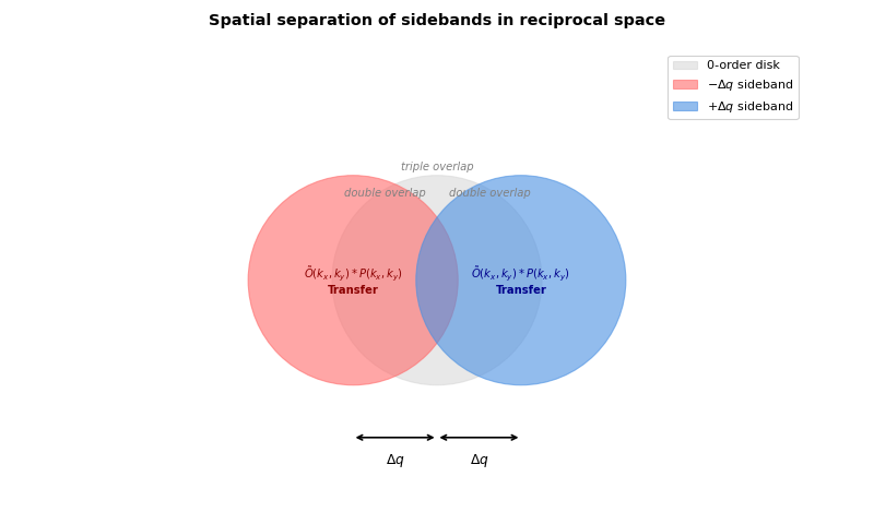
Important
This is NOT a diffraction pattern! Individual diffraction patterns recorded at each scan position do NOT show these three disks. At one scan position, only the interference pattern \(I(\mathbf{k}; \mathbf{R})\) is visible - a single 2D intensity distribution on the detector.
These diagrams show the structure of \(G(\mathbf{k}, \mathbf{Q})\) - a mathematical object created by Fourier transforming over all scan positions. Since \(G(\mathbf{k}, \mathbf{Q})\) is 4D, we visualize it by showing 2D slices or projections. The “three disks” represent different components that emerge in this transformed space: the center disk (autocorrelation at \(\mathbf{Q} = 0\)), and the two sidebands at \(\mathbf{Q} = \pm \mathbf{k}\) (containing object information). The sidebands exist only after processing the entire 4D dataset - they are not visible in any single measurement.
Phase extraction from single sideband
Why only one sideband is needed
The two sidebands (at \(\mathbf{Q} = +\mathbf{k}\) and \(\mathbf{Q} = -\mathbf{k}\)) contain the same information, just complex-conjugated. Keeping both causes interference and introduces redundancy. Selecting only one sideband produces a clean, linear signal. This is the reason for the term “single sideband.”
The complete SSB workflow
What is actually detected is the total intensity pattern—the sidebands at \(\pm \Delta q\) are not directly visible as separate entities. They exist mathematically as components of the Fourier decomposition of the recorded intensity, mixed together with the autocorrelation terms. The spatial separation discussed earlier refers to how these terms separate in reciprocal space after Fourier analysis.
SSB reconstructs the entire field of view simultaneously
Because SSB requires Fourier transforming over all scan positions, it reconstructs the entire field of view simultaneously, not individual spots. SSB cannot be performed on a single diffraction pattern—the full 4D dataset is required. The phase map \(\phi(x,y)\) that emerges covers the complete scanned area.
Step 1: Identify minimal sideband overlap
When the probe scan step size is large enough, sidebands separate cleanly with minimal overlap:
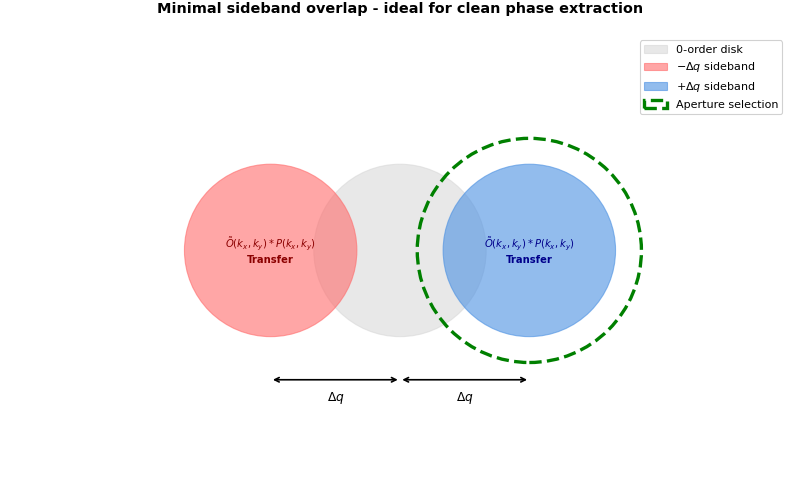
This shows the \(G(\mathbf{k}, \mathbf{Q})\) space with minimal sideband overlap (achieved when scan step size is large enough). A circular aperture (shown in green) is drawn around one sideband. The aperture size trades off resolution (smaller aperture, lower resolution) versus signal-to-noise ratio (larger aperture, more signal). This aperture selection happens in the transformed \((\mathbf{k}, \mathbf{Q})\) space after Fourier transforming over all scan positions, not on individual diffraction patterns.
Step 2: Crop and shift sideband to center
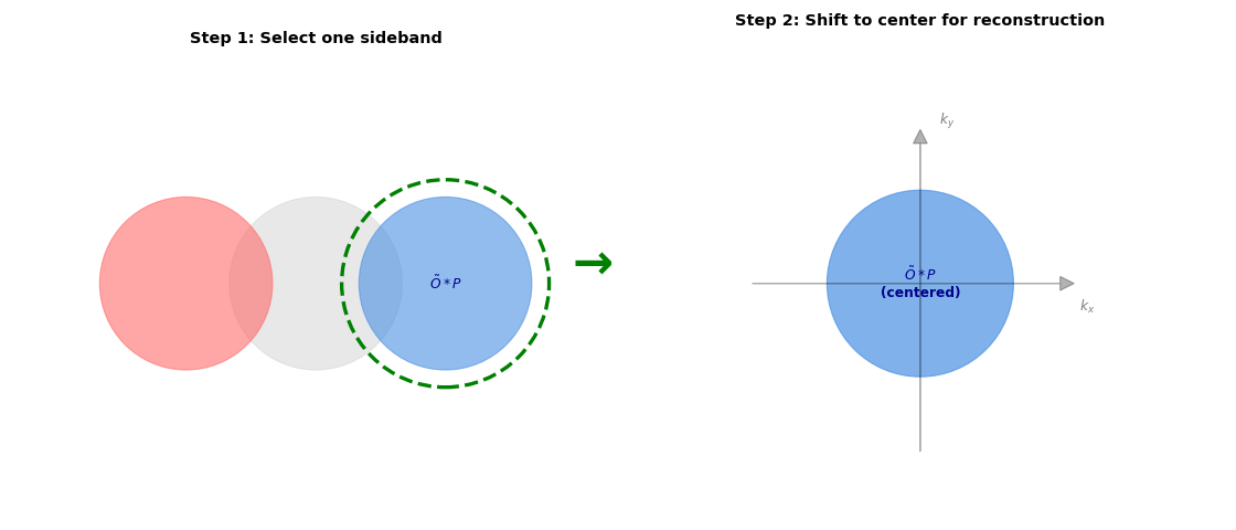
These diagrams show operations in \(G(\mathbf{k}, \mathbf{Q})\) space (after Fourier transforming over all scan positions). Left: aperture selection isolates one sideband. Right: the selected sideband shifted to center for reconstruction.
After Fourier transforming over scan positions, the sideband at \(\mathbf{Q} = +\mathbf{k}\) contains the object-probe convolution. An aperture \(A(\mathbf{Q})\) in \((\mathbf{k}, \mathbf{Q})\) space isolates this sideband:
With sufficient separation (minimal overlap case), the aperture primarily captures:
Shifting the sideband to center (setting \(\mathbf{Q}' = \mathbf{Q} - \mathbf{k}\) for the right sideband at \(\mathbf{Q} = +\mathbf{k}\)):
Warning
Critical approximation: The second \(\approx\) above is a strong assumption that requires:
Localized probe in k-space: The object’s spectrum \(\tilde{O}(\mathbf{k})\) varies slowly over the support of the probe kernel, so inside the aperture \(\tilde{O}(\mathbf{k})\) is almost constant on the scale of the probe kernel
Convolution behaves like multiplication: \(\tilde{O}(\mathbf{k}) * P(\mathbf{k}) \approx \tilde{O}(\mathbf{k}) |P(\mathbf{k})|^2\)
This is where SSB can break. When NOT true (sharp object features, strong phase variations, thick samples), the approximation fails and SSB produces artifacts, contrast errors, or frequency-dependent distortion. Your derivation is correct given this extra assumption. Treat this in your head as “this is where SSB can break.”
Step 3: Divide by the probe
Now centered at the origin, the sideband contains approximately \(|P(\mathbf{k})|^2 \tilde{O}(\mathbf{k})\). Dividing by the probe intensity isolates the object:
The probe \(P(\mathbf{k})\) must be known (measured from vacuum or constructed analytically). This division recovers the object’s Fourier content without iteration.
Step 4: Inverse Fourier transform back to real space
After dividing by the probe, we have \(\tilde{O}(\mathbf{k})\) in Fourier space. But remember, we’re still in the mixed \((\mathbf{k}, \mathbf{Q})\) representation. We need to inverse Fourier transform back over \(\mathbf{Q}\) to return to real space coordinates \(\mathbf{r} = (x, y)\):
This recovers the phase component of the object transmission function in real space.
What do we actually get?
Under the weak-phase approximation \(O(x,y) \approx 1 + i\phi(x,y)\), the sideband isolation removed the constant term (which stayed in the center disk at \(\mathbf{Q} = 0\)). The reconstructed quantity \(o(x,y)\) contains only the phase-dependent part:
Taking the imaginary part gives the phase directly:
This gives the object’s phase. Here \((x,y)\) are real-space coordinates on the sample, not scan positions. SSB directly recovers \(\phi(x,y)\) without iteration or integration. The weak-phase approximation makes this simple division-based reconstruction possible.
Note
In practice, the implementation processes data at each scan position and produces a stack of phase reconstructions (one per scan position), which are then typically averaged for the final result. See Optimizing probe parameters for how this stack is used in optimization.
Note
Caveats on recovered phase:
DC content lost: The constant term (overall phase offset and slow background) is lost when the center disk is discarded. Absolute offset and very low-frequency behavior are not well constrained, similar to DPC.
Regularization in practice: Practitioners often apply regularization or filtering in frequency space to improve signal-to-noise ratio and stability.
Summary: Why SSB is fast
All four SSB steps are linear operations:
Fourier transform over scan positions \(\mathbf{R} \to \mathbf{Q}\) (separates sidebands in \(G(\mathbf{k}, \mathbf{Q})\))
Aperture selection in \((\mathbf{k}, \mathbf{Q})\) space (isolates one sideband, suppresses conjugate)
Divide by probe \(|P(\mathbf{k})|^2\) (removes probe modulation to get \(\tilde{O}(\mathbf{k})\))
Inverse Fourier transform \(\mathbf{k} \to \mathbf{r}\) (get \(o(\mathbf{r})\), extract \(\phi = \text{Im}[o]\))
No iterative solver. No nonlinear optimization. No thousands of ePIE iterations. Just linear algebra. This simplicity makes SSB fast and robust to initialization errors.
Probe specification and aberration measurement
What probe information does SSB need?
SSB reconstruction requires knowing the probe function \(P(k_x, k_y)\) to perform the division step in reciprocal space. The probe function consists of two parts:
where \(A(k_x, k_y)\) is the aperture modulus (amplitude, typically a sharp circular cutoff at \(k_{\text{max}}\)) and \(\chi(k_x, k_y)\) is the aberration phase function encoding optical aberrations.
Simplified probe assumption for highly corrected microscopes
For modern aberration-corrected microscopes (Cs-corrected systems), most higher-order aberrations are negligible. In this case, a highly simplified probe model can be used:
where:
\(C_1\) is the defocus (typically the only significant aberration)
\(\lambda\) is the electron wavelength
\(k = \sqrt{k_x^2 + k_y^2}\) is the radial coordinate in reciprocal space
SSB requires accurate knowledge of the convergence angle to properly define \(k_{\text{max}}\).
Fortunately, the convergence angle is usually stable and easily obtained from the microscope settings.
General shape of the probe aperture
A circular, uniform aperture is usually a good approximation:
Unless your condenser system is misaligned or your aperture is damaged, this is safe.
Near-zero defocus
For near-zero defocus conditions:
This is one of the most important parts. SSB is extremely sensitive to defocus error, but if yours really is near zero, guessing “0” is fine.
Small higher-order aberrations
If your microscope is well-corrected (Cs-corrector), then C3, C5… are small enough that:
This is not perfect, but usually good enough to do SSB without horrible artifacts.
When more detailed probe measurement is needed
For uncorrected microscopes or when higher accuracy is required, the full aberration phase \(\chi(k_x, k_y)\) must be measured. This includes defocus, spherical aberration, astigmatism, coma, and higher-order terms.
Why aberrations appear in the sideband
Because the selected sideband \(S(\mathbf{k})\) depends directly on the probe:
it includes both the probe amplitude \(|P(\mathbf{k})|\) and the aberration phase \(\chi(\mathbf{k})\) (contained in \(P = A e^{i\chi}\)). The phase and shape of \(S(\mathbf{k})\) directly encode \(\chi(\mathbf{k})\).
Breaking the chicken-and-egg problem
SSB faces a fundamental issue: to extract phase, the probe must be known, but to measure the probe, the object must be known. SSB breaks this cycle using two separate measurements:
First, measure the probe on a simple reference (vacuum, amorphous film) where the object is known
Then, use that measured probe to extract phase from unknown samples
For a reference with known \(\tilde{O}(k_x, k_y)\), the probe is recovered from the sideband:
Once measured, this probe can be used for all subsequent reconstructions in the same imaging session (assuming the probe doesn’t change).
Required conditions for accurate measurement
SSB provides clean probe aberration measurements under specific conditions:
Simple object: Vacuum edge, uniform amorphous carbon, or ultrathin film allow accurate estimation of \(\tilde{O}(k_x, k_y)\) for division
High signal-to-noise ratio: Phase extraction requires low noise to resolve fine details of \(\chi(k_x, k_y)\)
Well-separated sidebands: The sideband must be far from the center disk and noise to avoid contamination from other terms
Coherent probe: Partially coherent or incoherent probes broaden the sideband and degrade phase resolution
Weak-phase approximation valid: Thick samples or strong-scattering materials violate the approximation and introduce errors
Negligible multiple scattering: Thick or crystalline samples scatter multiple times, corrupting the sideband
When all these conditions hold, division by the object term yields a clean \(P(k_x, k_y)\), and the aberrations can be reliably extracted.
Parameters that cannot be reliably estimated
Even with a highly corrected microscope, certain parameters introduce artifacts if guessed incorrectly. These are the danger areas:
Residual astigmatism
Even tiny astigmatism distorts the sideband shape and can introduce anisotropic artifacts. This cannot be blindly guessed.
Residual coma
Coma shifts the probe and skews the sideband. If small, SSB survives; if moderate, it breaks.
Finite source size and partial coherence
If the illumination is not coherent enough, the sideband contrast decreases and blurs. Guessing wrong means SSB incorrectly amplifies noise on division.
Defocus drift
If the defocus changes during the scan due to stage drift or thermal instability, the probe varies across the field of view. SSB assumes a constant probe, so this introduces systematic errors that cannot be corrected by a single probe measurement.
Practical guide for using SSB
Required microscope parameters
SSB reconstruction requires these experimental parameters:
Convergence angle (α): Defines \(k_{\text{max}}\) for the probe aperture (units: mrad)
Acceleration voltage: Determines the electron wavelength \(\lambda\) (units: keV → Å)
Camera length: Converts detector pixels to reciprocal space units (mrad)
These are standard microscope parameters that should be stable and easy to obtain from your instrument.
Note
Unit conversions:
Convergence angle in mrad → \(k_{\text{max}}\) in Ų: \(k_{\text{max}} = \alpha / \lambda\) where \(\alpha\) is in radians
Acceleration voltage in keV → wavelength in Å: \(\lambda = \frac{12.398}{\sqrt{E(E + 1022)}}\) where \(E\) is in keV
Example: 60 keV → λ = 0.0487 Å, 34 mrad → k_max = 0.698 Ų
Method 1: Use a vacuum region inside your scan
This is the easiest and most robust method. If your scan area includes vacuum (no sample), the SSB sideband over vacuum directly measures the probe:
because over vacuum, \(O(x,y) = 1\) (no object), so \(\tilde{O} = \delta(k)\) and the sideband equals the probe.
Procedure:
Collect 4D-STEM data with part of the scan over vacuum (sample edge or hole)
Process the vacuum region separately to extract \(P(k_x, k_y)\)
Use this measured probe for all sample positions in the same dataset
This provides a real probe measurement without estimation. The vacuum measurement captures all aberrations, including residual astigmatism, coma, and defocus, as they actually exist at the time of data acquisition.
Method 2: Thin amorphous reference film
If no vacuum is available, use a uniform thin amorphous carbon or silicon nitride film where \(\phi(x,y) \approx\) constant. The sideband over this region approximates the probe with only a weak, slowly varying phase offset.
Method 3: Simple analytical probe (for quick tests)
For rapid prototyping or when accuracy is not critical, construct an analytical probe from microscope parameters:
where:
\(A(k) = 1\) for \(k < k_{\text{max}}\), 0 otherwise (from convergence angle)
\(\chi(k) = \pi C_1 \lambda k^2\) (defocus only, if near zero set \(C_1 = 0\))
This works for highly corrected microscopes but ignores residual aberrations.
Processing workflow
Load 4D-STEM dataset: \(I(\mathbf{k}; \mathbf{R})\) where \(\mathbf{R}\) are scan positions, \(\mathbf{k}\) are detector pixels
Measure or construct probe \(P(\mathbf{k})\) using vacuum region, reference film, or analytical model
Fourier transform over scan positions: Transform the 4D data \(I(\mathbf{k}; \mathbf{R})\) over the \(\mathbf{R}\) dimensions to create \(G(\mathbf{k}, \mathbf{Q})\), where \(\mathbf{Q}\) is spatial frequency
Select one sideband: Apply circular aperture \(A(\mathbf{Q} - \mathbf{k})\) in \((\mathbf{k}, \mathbf{Q})\) space to isolate sideband at \(\mathbf{Q} = \pm \mathbf{k}\)
Shift sideband to center: Re-center by setting \(\mathbf{Q}' = \mathbf{Q} \mp \mathbf{k}\) to get \(S(\mathbf{k})\)
Divide by probe intensity: \(\tilde{O}(\mathbf{k}) = S(\mathbf{k}) / |P(\mathbf{k})|^2\)
Inverse Fourier transform: Transform \(\tilde{O}(\mathbf{k})\) back to real space to get \(o(x,y) \approx i\phi(x,y)\)
Extract phase: \(\phi(x,y) = \text{Im}[o(x,y)]\)
The vacuum region method (Method 1) for measuring the probe is strongly recommended because it captures actual experimental conditions without guesswork.
Advantages and limitations
Advantages:
Direct, non-iterative phase extraction via linear operations
Simple workflow once probe is known
Works well for thin samples under weak-phase approximation
Easy to measure probe aberrations from reference samples
Entire field of view reconstructed simultaneously
Limitations:
Requires weak-phase approximation (thin samples, \(\phi \ll 1\))
Resolution limited by sideband separation and signal-to-noise ratio
Probe knowledge critical—errors in aberration coefficients cause artifacts
Lower redundancy exploitation compared to iterative ptychography
Phase contrast transfer function falls off at high spatial frequencies
Implementation in quantem
The following sections describe how the conceptual framework above is implemented in the quantem library. The implementation follows the same physics but uses computational notation and provides practical tools for real data analysis.
Probe representation
The probe function \(P(\mathbf{k})\) from Probe specification and aberration measurement is implemented as:
where \(A(\mathbf{k})\) is the aperture function (soft or hard-edged circular) and \(\chi(\mathbf{k})\) is the aberration phase function.
Aberration function expansion
The aberration function \(\chi(\mathbf{k})\) is parameterized using Zernike-like polynomial expansion:
where:
\(\lambda\) is the electron wavelength
\(C_{nm}\) are the aberration coefficients (e.g., \(C_{10}\) = defocus, \(C_{12}\) = astigmatism, \(C_{30}\) = spherical aberration)
\(k = |\mathbf{k}|\) and \(\phi = \arctan(k_y/k_x)\) are polar coordinates
\(\phi_{nm}\) are azimuthal angles for non-rotationally symmetric aberrations
The most important aberration terms are:
where \(C_{10}\) is defocus, \(C_{12}\) is two-fold astigmatism with angle \(\phi_{12}\), and \(C_{30}\) is third-order spherical aberration. These are the same aberration coefficients discussed in the “Probe specification” section earlier.
SSB transfer function
The implementation uses a transfer function \(\Gamma(\mathbf{Q}, \mathbf{k})\) (sometimes called the deconvolution kernel) to perform sideband isolation and probe division. This implements the conceptual steps from Phase extraction from single sideband (aperture selection, shift, divide) in a single mathematical operation.
Three deconvolution kernel options
The deconvolution_kernel parameter selects different reconstruction methods:
1. ‘none’ (Bright-field imaging)
No deconvolution applied. Simply returns the measured bright-field intensity without phase extraction. Fast but provides no phase information.
2. ‘quadratic’ (Parallax method)
A simplified approximation that’s faster to compute but less accurate than full SSB. Useful for hyperparameter optimization where speed matters.
3. ‘full’ (Complete SSB - default)
This implements the complete SSB method from Phase extraction from single sideband:
First term: selects the \(+\mathbf{k}\) sideband
Subtraction: suppresses the \(-\mathbf{k}\) conjugate sideband (removes twin-image artifacts)
The form includes implicit probe division
The asymmetric form (subtraction) gives better noise properties than the symmetric form (addition).
Normalization
To prevent numerical instabilities from division by near-zero values, the operator is normalized:
where \(\epsilon = 10^{-8}\) is a regularization parameter that prevents division by zero when the probe is weak.
Reconstruction workflow
The implementation follows the conceptual workflow from Phase extraction from single sideband:
Data preparation
Load 4D-STEM dataset \(I(\mathbf{k}; \mathbf{R})\) with shape
(scan_x, scan_y, detector_x, detector_y)Identify bright-field disk using center-of-mass or fit_probe_circle
Extract BF intensities within aperture mask
Probe specification
Define the probe \(P(\mathbf{k})\) using one of the three methods from Practical guide for using SSB:
Code example: Probe specification
# Method 1: From vacuum region (recommended)
# Method 2: From thin amorphous film
# Method 3: Analytical from microscope parameters

cmplx_probe = evaluate_probe(
    alpha, phi,               # Polar coordinates in k-space
    semiangle_cutoff,         # Convergence angle [mrad]
    wavelength,               # Electron wavelength [Å]
    aberration_coefs={        # Aberration coefficients [Å]
        'C10': 0,             # Defocus (near zero)
        'C12': 10,            # Astigmatism magnitude
        'phi12': 0.5,         # Astigmatism angle [rad]
    }
)
Applying the transfer function
For each scan position, apply the transfer function \(\Gamma(\mathbf{Q}, \mathbf{k})\) which implements the steps from Phase extraction from single sideband:
Fourier transform over scan positions: Transform the 4D dataset \(I(\mathbf{k}; \mathbf{R})\) over the scan coordinate \(\mathbf{R}\) to create \(G(\mathbf{k}, \mathbf{Q})\) from Sideband formation in reciprocal space:
\[G(\mathbf{k}, \mathbf{Q}) = \mathcal{F}_{\mathbf{R} \to \mathbf{Q}}[I(\mathbf{k}; \mathbf{R})]\]In the implementation, this is
torch.fft.fft2(vbf_stack)wherevbf_stackis the bright-field intensity at each scan position.Apply \(\Gamma(\mathbf{Q}, \mathbf{k})\) to isolate and deconvolve one sideband:
\[\tilde{O}(\mathbf{Q}) = G(\mathbf{k}, \mathbf{Q}) \cdot \Gamma(\mathbf{Q}, \mathbf{k})\]This multiplication in Fourier space implements the aperture selection, shift, and probe division.
Inverse Fourier transform to get object \(o(\mathbf{r})\):
\[o(\mathbf{r}) = \mathcal{F}_{\mathbf{Q} \to \mathbf{r}}^{-1}[\tilde{O}(\mathbf{Q})]\]In code:
torch.fft.ifft2(fourier_factor)Extract phase: \(\phi(\mathbf{r}) = \text{Im}[o(\mathbf{r})]\) or equivalently
corrected_stack.angle()
The final result is averaged over all positions for improved signal-to-noise.
Scan-detector rotation correction
As mentioned in the practical guide, there can be a rotation \(\theta\) between the scan coordinate system (probe motion) and the detector coordinate system (diffraction pattern recording). The implementation corrects for this:
where \(\theta\) is in radians for the mathematical operations.
Note
Angle units: Internal calculations use radians, but the user-facing API accepts degrees for convenience. The function parameters are:
rotation_angle_deg: User input in degrees (e.g., 0.38°)rotation_angle_rad: Internal computation in radians (e.g., 0.0066 rad)
Conversion: \(\theta_{\text{rad}} = \theta_{\text{deg}} \times \pi / 180\)
This rotation is applied to the reciprocal space grid before probe evaluation, ensuring the reconstructed object aligns with the scan coordinate system. The rotation angle can be optimized (see next section).
Optimizing probe parameters
What’s being optimized?
SSB needs to know the probe’s aberrations (defocus, astigmatism) and the rotation angle between scan and detector coordinates. If you don’t have a vacuum region to measure these directly, the code can guess-and-check to find the best values.
What gets adjusted:
C₁₀ (defocus): How far out of focus the probe is
C₁₂ (astigmatism): How much the probe is stretched in one direction
φ₁₂ (astigmatism angle): Which direction it’s stretched
θ (rotation): How much the scan grid is rotated relative to the detector
The trick: Self-consistency check
As discussed in Phase extraction from single sideband, SSB processes the entire 4D dataset together. The output is a stack of phase images - one 2D image \(\phi(x,y)\) for each scan position. So from a 100×100 scan, you get 100×100 different reconstructions of the sample phase.
Key insight: The sample itself doesn’t move - only the probe moves across it. So all 100×100 reconstructed images should show the same sample structure if your probe parameters are correct.
How this works for optimization:
For each detector pixel \((k_x, k_y)\), SSB does an FFT over how intensity varies across all scan positions \((R_x, R_y)\). Then it divides by \(|P(\mathbf{k})|^2\) using your probe parameters. If those parameters are wrong, you’re dividing by the wrong probe - this creates errors that vary from position to position.
Correct parameters (right C₁₀, C₁₂, θ): All phase maps agree → low variance
Wrong parameters: Each scan position has different artifacts → high variance
The optimization finds probe parameters that minimize this variance across all reconstructed phase maps.
The optimization:
Try some values for C₁₀, C₁₂, φ₁₂, θ
Reconstruct phase from each scan position separately
Compare how similar all the reconstructions are
If they disagree a lot → bad parameters, try different values
If they agree well → good parameters, keep these!
Repeat until you find the parameters that make all reconstructions match best
What “variance” means here:
Imagine you reconstruct the phase 100 times (once from each scan position). Now at pixel (x,y) in your image, you have 100 different phase values. “Variance” measures how spread out these 100 values are:
Low variance: All 100 values are nearly the same (e.g., all around 0.5 radians) → reconstructions agree → good parameters
High variance: Values are all over the place (0.2, 0.7, 0.1, 0.9…) → reconstructions disagree → bad parameters
The math computes this for every pixel, then adds up the variance across the whole image. The goal is to find probe parameters that minimize this total disagreement.
where \(\phi_n\) is the phase at that pixel from position \(n\), and \(\bar{\phi}\) is the average phase across all positions.
Important limitation: This only works with good detector sampling (≥64×64 pixels, ideally 128×128+). With only 12×12 pixels, there’s not enough information to reliably find the right parameters.
Optimization algorithm
The implementation uses Optuna with Tree-structured Parzen Estimator (TPE) sampling:
Parameter Space:
For aberration-corrected microscopes (recommended starting ranges):
\[\mathbf{\Theta} = \{C_{10} \in [-100, 100]\text{ Å}, \, C_{12} \in [0, 50]\text{ Å}, \, \phi_{12} \in [-\pi/2, \pi/2], \, \theta \in [-10°, 10°]\}\]For uncorrected microscopes or initial exploration, use wider ranges: \(C_{10} \in [-400, 400]\) Å, \(\theta \in [-180°, 180°]\), and increase \(C_{12}\) range to [0, 100] Å.
Objective Function:
def objective(trial):
    # Sample parameters
    C10 = trial.suggest_float('C10', -400, 400)
    C12 = trial.suggest_float('C12', 0, 100)
    phi12 = trial.suggest_float('phi12', -np.pi/2, np.pi/2)
    theta = trial.suggest_float('rotation_angle_rad', -np.pi, np.pi)

    # Reconstruct with these parameters
    reconstruct(aberration_coefs={'C10': C10, 'C12': C12, 'phi12': phi12},
               rotation_angle_rad=theta)

    # Return variance loss
    return variance_loss()
Optimization Loop:
Run for \(N_{\text{trials}}\) iterations (typically 50-100) to find:
\[\mathbf{\Theta}^* = \arg\min_{\mathbf{\Theta}} \mathcal{L}(\mathbf{\Theta})\]
Code organization
Module structure
The SSB algorithm is implemented across two main modules:
1. complex_probe.py
Contains core mathematical operators:
gamma_factor(): Computes the SSB transfer function \(\Gamma(\mathbf{Q}, \mathbf{k})\)evaluate_probe(): Evaluates complex probe with aberrationsaberration_surface(): Computes aberration phase surfaceaperture(): Soft/hard aperture functionsspatial_frequencies(): Generates Fourier grids with rotation
2. direct_ptychography.py
Orchestrates the reconstruction pipeline:
DirectPtychographyclass: Main interfacefrom_dataset4d(): Constructor from 4D-STEM datareconstruct(): Performs SSB reconstructionoptimize_hyperparameters(): Optuna-based optimization_compute_gamma_operator(): Wrapper for transfer function computationvariance_loss(): Self-consistency metric
Key implementation functions
Transfer function computation
Code example: Transfer function computation
def gamma_factor(
    qmks: tuple[Tensor, Tensor],      # (q - k) coordinates
    qpks: tuple[Tensor, Tensor],      # (q + k) coordinates
    cmplx_probe_at_k: Tensor,         # P(k)
    wavelength: float,
    semiangle_cutoff: float,
    soft_edges: bool,
    aberration_coefs: dict,
    angular_sampling: tuple,
    asymmetric_version: bool = True,
    normalize: bool = True,
) -> Tensor:
    """
    Compute the SSB transfer function Γ(Q,k).

    Returns:
        Γ(q,k) = P(q-k)P*(k) - P*(q+k)P(k)  [asymmetric]
        or
        Γ(q,k) = P(q-k)P*(k) + P*(q+k)P(k)  [symmetric]
    """
    # Evaluate probe at q-k
    probe_m = evaluate_probe(q_m * wavelength, phi_m, ...)

    # Evaluate probe at q+k
    probe_p = evaluate_probe(q_p * wavelength, phi_p, ...)

    # Compute transfer function Γ
    if asymmetric_version:
        gamma = probe_m * cmplx_probe_at_k.conj() - probe_p.conj() * cmplx_probe_at_k
    else:
        gamma = probe_m * cmplx_probe_at_k.conj() + probe_p.conj() * cmplx_probe_at_k

    # Normalize
    if normalize:
        gamma /= gamma.abs().clamp(min=1e-8)

    return gamma.conj()
Probe evaluation
Code example: Probe evaluation
def evaluate_probe(
    alpha: Tensor,                 # Radial angles [rad]
    phi: Tensor,                   # Azimuthal angles [rad]
    semiangle_cutoff: float,       # Aperture size [mrad]
    angular_sampling: tuple,       # Pixel size in angle space
    wavelength: float,             # Wavelength [Å]
    aberration_coefs: dict,        # Aberration coefficients
) -> Tensor:
    """
    Evaluate complex probe function: P(k) = A(k) exp[-iχ(k)]
    """
    # Aperture function (soft or hard edge)
    aperture = compute_aperture(alpha, semiangle_cutoff, ...)

    # Aberration phase
    chi = aberration_surface(alpha, phi, wavelength, aberration_coefs)

    # Complex probe
    return aperture * torch.exp(-1j * chi)
Reconstruction pipeline
Code example: Reconstruction pipeline
def reconstruct(
    self,
    aberration_coefs: dict = None,
    rotation_angle_rad: float = None,
    upsampling_factor: int = 1,
    deconvolution_kernel: str = 'full',  # 'full'=SSB, 'quadratic'=parallax
    max_batch_size: int = None,
):
    """
    Perform SSB/parallax/BF reconstruction.
    """
    # Setup coordinate grids with rotation
    kxa, kya = spatial_frequencies(self.gpts, self.sampling, rotation_angle)
    qxa, qya = upsampled_frequencies(upsampling_factor)

    # Compute complex probe at all k-vectors
    cmplx_probe = evaluate_probe(alpha, phi, ...)

    # Process each scan position in batches
    for batch_idx in batcher:
        # Get bright-field data in Fourier space
        vbf_fourier = torch.fft.fft2(self.vbf_stack[batch_idx])

        # Compute transfer function Γ(Q,k) for this batch
        operator = self._compute_gamma_operator(
            kxa, kya, qxa, qya,
            aberration_coefs, cmplx_probe, batch_idx
        )

        # Apply transfer function (deconvolution)
        fourier_factor = vbf_fourier * operator

        # Inverse FFT to get real-space reconstruction
        corrected_stack[batch_idx] = torch.fft.ifft2(fourier_factor)

    # Extract phase for SSB
    self.corrected_stack = corrected_stack.angle()

    # Mean across all positions
    self.mean_corrected_bf = self.corrected_stack.mean(dim=0)

    return self
Usage examples
These examples demonstrate how to apply the concepts from Why SSB?, Sideband formation in reciprocal space, and Practical guide for using SSB using the quantem library.
Method 1: Extract probe from vacuum region (recommended)
If your scan includes vacuum (sample edge or hole), measure the probe directly:
Code example: Vacuum probe extraction
import quantem as em
import numpy as np

# Load 4D-STEM dataset
dataset = em.io.read_emdfile_to_4dstem('data.h5')

# Method 1: Identify vacuum region in your scan
# (assume vacuum is in the top-left corner, positions 0-10)
vacuum_positions = dataset[0:10, 0:10]  # Adjust to your data

# Extract probe from vacuum region
# Over vacuum, O(x,y) = 1, so the sideband directly measures P(k)
vacuum_probe = extract_probe_from_vacuum(
    vacuum_positions,
    energy=60e3,
    semiangle_cutoff=34.0,
)

# Use measured probe for reconstruction on sample region
direct_ptycho = em.diffractive_imaging.DirectPtychography.from_dataset4d(
    dataset,
    energy=60e3,
    semiangle_cutoff=34.0,
    measured_probe=vacuum_probe,    # Use measured probe
    device='mps',
)

result = direct_ptycho.reconstruct(deconvolution_kernel='full')
em.visualization.show_2d(result.obj, title='Phase [rad]')
Method 3: Analytical probe from microscope parameters
For quick tests when vacuum is not available:
Code example: Analytical probe reconstruction
import quantem as em

# Load 4D-STEM dataset
dataset = em.io.read_emdfile_to_4dstem('data.h5')

# Initialize with analytical probe from microscope parameters
direct_ptycho = em.diffractive_imaging.DirectPtychography.from_dataset4d(
    dataset,
    energy=60e3,                     # 60 keV
    semiangle_cutoff=34.0,           # 34 mrad convergence angle
    aberration_coefs={'C10': 0},     # Near-zero defocus
    rotation_angle_deg=0,            # Assume aligned
    device='mps',                    # 'mps' (Apple), 'cuda' (NVIDIA), or 'cpu'
)

# Reconstruct the object phase
result = direct_ptycho.reconstruct(
    deconvolution_kernel='full',     # Full SSB deconvolution
)

# The result is the phase map φ(x,y) from the conceptual section
em.visualization.show_2d(result.obj, title='Phase [rad]')
With hyperparameter optimization (recommended)
When you don’t have a reference measurement, optimize the probe parameters from your data using the self-consistency loss described above:
Code example: Hyperparameter optimization
import optuna
import numpy as np

# Optimize aberrations and rotation angle
# Use narrow ranges around expected values for faster convergence
sampler = optuna.samplers.TPESampler(seed=42)
direct_ptycho.optimize_hyperparameters(
    aberration_coefs={
        'C10': (-100, 100),           # Search defocus [Å] - narrow for corrected scope
        'C12': (0, 50),               # Search astigmatism [Å]
        'phi12': (-np.pi/2, np.pi/2), # Astigmatism angle [rad]
    },
    rotation_angle_deg=(-10, 10),     # Search rotation [degrees] - typically small
    deconvolution_kernel='quadratic', # Use faster parallax method for optimization
    sampler=sampler,
    n_trials=30,                      # 30 trials usually sufficient with narrow ranges
)

# Note: For wider exploration (uncorrected microscope, uncertain defocus):
# Use C10: (-400, 400), rotation_angle_deg: (-180, 180), n_trials: 50-100

# Results show optimized parameters
print(f"Optimized C10: {direct_ptycho._optimized_parameters['C10']:.1f} Å")
print(f"Optimized C12: {direct_ptycho._optimized_parameters['C12']:.1f} Å")
print(f"Optimized rotation: {direct_ptycho._optimized_parameters['rotation_angle_deg']:.2f}°")

# Reconstruct with optimized parameters
result = direct_ptycho.reconstruct_with_optimized_parameters(
    deconvolution_kernel='full',      # Full SSB for final result
)

# This is the best estimate of φ(x,y) given your data
em.visualization.show_2d(result.obj, title='Optimized phase [rad]')
Comparing reconstruction methods
Compare different approximations discussed in Phase extraction from single sideband:
Code example: Method comparison (BF vs Parallax vs SSB)
# 1. Bright-field: No deconvolution, intensity only
bf_result = direct_ptycho.reconstruct_with_optimized_parameters(
    deconvolution_kernel='none',
    use_center_of_mass_weighting=False,
)

# 2. Parallax: Quadratic approximation to full SSB
parallax_result = direct_ptycho.reconstruct_with_optimized_parameters(
    deconvolution_kernel='quadratic',
)

# 3. SSB: Full deconvolution as described conceptually
ssb_result = direct_ptycho.reconstruct_with_optimized_parameters(
    deconvolution_kernel='full',
)

# Compare amplitudes and phases
em.visualization.show_2d([
    [np.abs(bf_result.obj), np.abs(parallax_result.obj), np.abs(ssb_result.obj)],
    [np.angle(bf_result.obj), np.angle(parallax_result.obj), np.angle(ssb_result.obj)]
], title=[
    ['BF amplitude', 'Parallax amplitude', 'SSB amplitude'],
    ['BF phase', 'Parallax phase', 'SSB phase']
])
This comparison shows:
BF: Fast but limited resolution, no deconvolution
Parallax: Faster approximation, good for optimization
SSB: Full reconstruction following the conceptual framework
References
Key papers on SSB and direct ptychography:
Ophus, C. (2019). Four-dimensional scanning transmission electron microscopy (4D-STEM): from scanning nanodiffraction to ptychography and beyond. Microscopy and Microanalysis, 25(3), 563-582.
Chen, Z., et al. (2021). Electron ptychography achieves atomic-resolution limits set by lattice vibrations. Science, 372(6544), 826-831.
Rodenburg, J. M., & Bates, R. H. T. (1992). The theory of super-resolution electron microscopy via Wigner-distribution deconvolution. Philosophical Transactions of the Royal Society A, 339(1655), 521-553.
Maiden, A. M., & Rodenburg, J. M. (2009). An improved ptychographical phase retrieval algorithm for diffractive imaging. Ultramicroscopy, 109(10), 1256-1262.