Quantum mechanics I

This page covers fundamental quantum mechanics, starting from first principles.

Note

What can be derived vs what are postulates

Quantum mechanics is built on several fundamental postulates (axioms that cannot be derived from more basic principles). These are:

  1. Wavefunction postulate: Systems are described by wavefunctions \(\psi(\mathbf{r}, t)\)

  2. Probability postulate: \(|\psi|^2\) gives the probability density

  3. Schrödinger equation: \(i\hbar \frac{\partial \psi}{\partial t} = \hat{H} \psi\) governs time evolution

  4. Operator postulate: Observables are represented by Hermitian operators

  5. Measurement postulate: Measuring gives eigenvalues with probabilities \(|c_n|^2\)

  6. Commutation relation: \([\hat{x}, \hat{p}] = i\hbar\) (fundamental quantum relation)

Everything else (uncertainty principle, eigenstate properties, orthogonality, etc.) can be mathematically derived from these postulates. This page shows both postulates and their derived consequences.

Wave-particle duality

Classical vs quantum description

What is the fundamental difference between classical and quantum mechanics?

In classical mechanics, we describe particles as having definite positions and momenta at all times. We describe their motion using Newton’s laws: \(\mathbf{F} = m\mathbf{a}\).

In quantum mechanics, we describe particles by wavefunctions \(\psi(\mathbf{r}, t)\) that encode probabilities. We see that the particle doesn’t have a definite position until measured. Instead, we find that \(|\psi(\mathbf{r}, t)|^2\) gives the probability density of finding the particle at position \(\mathbf{r}\) at time \(t\).

Why do we need quantum mechanics?

We observe that classical mechanics fails at atomic scales. At these scales:

  • We see that particles exhibit wave-like behavior (diffraction, interference)

  • We find that energy is quantized (only certain discrete values allowed)

  • We cannot simultaneously know position and momentum precisely (uncertainty principle)

  • We observe that particles can tunnel through barriers classically forbidden

Quantum mechanics is the framework that correctly describes what we observe in nature at atomic and subatomic scales.

de Broglie relation

What is the de Broglie wavelength?

Louis de Broglie (1924) proposed that all matter has wave properties. We see that a particle with momentum \(p\) has an associated wavelength:

\[\lambda = \frac{h}{p}\]

where \(h = 6.626 \times 10^{-34}\) J·s is Planck’s constant.

Physical meaning: We observe that higher momentum gives shorter wavelength and more particle-like behavior. Lower momentum gives longer wavelength and more wave-like behavior.

Schrödinger equation

Time-dependent Schrödinger equation

What is the fundamental equation of quantum mechanics?

The time-dependent Schrödinger equation describes how we observe wavefunctions to evolve:

\[i\hbar \frac{\partial \psi}{\partial t} = \hat{H} \psi\]
Here, we have:
  • \(\psi(\mathbf{r}, t)\): wavefunction (complex-valued)

  • \(\hbar = h/(2\pi)\): reduced Planck constant

  • \(\hat{H}\): Hamiltonian operator (total energy operator)

For a particle in a potential \(V(\mathbf{r})\), we write:

\[i\hbar \frac{\partial \psi}{\partial t} = -\frac{\hbar^2}{2m} \nabla^2 \psi + V(\mathbf{r}) \psi\]

We see that the first term is kinetic energy, the second is potential energy.

What does the wavefunction mean physically?

We observe that the wavefunction \(\psi(\mathbf{r}, t)\) itself is not directly observable. We find that its squared magnitude gives the probability density:

\[P(\mathbf{r}, t) = |\psi(\mathbf{r}, t)|^2\]

This means: the probability of finding the particle in a small volume \(dV\) around position \(\mathbf{r}\) is \(|\psi(\mathbf{r}, t)|^2 dV\).

We require that the wavefunction must be normalized:

\[\int |\psi(\mathbf{r}, t)|^2 d^3r = 1\]

(The particle must be somewhere!)

The superposition principle

What is the superposition principle?

We see one of the most fundamental principles in quantum mechanics: if \(\psi_1\) and \(\psi_2\) are solutions to the Schrödinger equation, then any linear combination is also a solution:

\[\psi = c_1 \psi_1 + c_2 \psi_2\]

where \(c_1\) and \(c_2\) are complex constants.

Physical meaning: We observe that a quantum system can exist in a superposition of multiple states simultaneously. The particle isn’t “in state 1” or “in state 2” — we see it’s in both at once until we measure it.

Why does superposition work?

We note that the Schrödinger equation is linear in \(\psi\). If \(\psi_1\) satisfies:

\[i\hbar \frac{\partial \psi_1}{\partial t} = \hat{H} \psi_1\]

and \(\psi_2\) satisfies:

\[i\hbar \frac{\partial \psi_2}{\partial t} = \hat{H} \psi_2\]

Then for \(\psi = c_1 \psi_1 + c_2 \psi_2\), we find:

\[i\hbar \frac{\partial \psi}{\partial t} = i\hbar \frac{\partial}{\partial t}(c_1 \psi_1 + c_2 \psi_2) = c_1 i\hbar \frac{\partial \psi_1}{\partial t} + c_2 i\hbar \frac{\partial \psi_2}{\partial t}\]
\[= c_1 \hat{H} \psi_1 + c_2 \hat{H} \psi_2 = \hat{H}(c_1 \psi_1 + c_2 \psi_2) = \hat{H} \psi\]

We see that the superposition \(\psi\) also satisfies the Schrödinger equation!

What does this mean for measurements?

If we have the system in a superposition \(\psi = c_1 \psi_1 + c_2 \psi_2\) where \(\psi_1\) and \(\psi_2\) are eigenstates with eigenvalues \(E_1\) and \(E_2\):

  • We find that measuring the energy will give either \(E_1\) or \(E_2\) (not both, not an average!)

  • We calculate the probability of getting \(E_1\): \(|c_1|^2/(|c_1|^2 + |c_2|^2)\)

  • We calculate the probability of getting \(E_2\): \(|c_2|^2/(|c_1|^2 + |c_2|^2)\)

This is what we observe as the essence of quantum mechanics: superposition before measurement, definite outcome after measurement.

Famous examples:

  • Electron going through double slits (we see superposition of “through left slit” and “through right slit”)

  • Schrödinger’s cat (superposition of “alive” and “dead” — though this is a thought experiment!)

  • Quantum computing: we work with qubits in superposition of |0⟩ and |1⟩

Where does the kinetic energy operator come from?

We see that the kinetic energy operator comes from quantum mechanical postulates and the correspondence principle.

Classical mechanics: We write kinetic energy as \(T = \frac{p^2}{2m}\) where \(p\) is momentum.

Quantum mechanics postulate: We have that physical observables become operators. Position \(\mathbf{r}\) stays as multiplication, but we find that momentum becomes a derivative:

\[\hat{\mathbf{p}} = -i\hbar \nabla\]

Why this form? We see that it ensures the de Broglie relation \(\lambda = h/p\) is satisfied.

First, we connect de Broglie to wave vector k:

We start from de Broglie’s relation:

\[\lambda = \frac{h}{p}\]

We use the definition of wave number \(k = 2\pi/\lambda\):

\[k = \frac{2\pi}{\lambda} = \frac{2\pi p}{h}\]

We use \(\hbar = h/(2\pi)\) (so \(h = 2\pi\hbar\)):

\[k = \frac{2\pi p}{2\pi\hbar} = \frac{p}{\hbar}\]

We rearrange to get:

\[\boxed{p = \hbar k}\]

We see this is the fundamental connection between momentum (particle picture) and wave vector (wave picture).

Now we verify the momentum operator gives this: For a plane wave \(\psi = e^{i\mathbf{k} \cdot \mathbf{r}}\), we find:

\[\hat{\mathbf{p}} \psi = -i\hbar \nabla e^{i\mathbf{k} \cdot \mathbf{r}} = -i\hbar (i\mathbf{k}) e^{i\mathbf{k} \cdot \mathbf{r}} = \hbar \mathbf{k} e^{i\mathbf{k} \cdot \mathbf{r}}\]

We see that the eigenvalue is \(\hbar \mathbf{k}\), which equals \(\mathbf{p}\) by the connection we just derived. Perfect consistency!

Kinetic energy operator: We replace classical \(p^2\) with operator \(\hat{p}^2\):

\[\hat{T} = \frac{\hat{p}^2}{2m} = \frac{1}{2m}(-i\hbar \nabla)^2 = \frac{1}{2m}(-\hbar^2 \nabla^2) = -\frac{\hbar^2}{2m} \nabla^2\]

where \(\nabla^2 = \frac{\partial^2}{\partial x^2} + \frac{\partial^2}{\partial y^2} + \frac{\partial^2}{\partial z^2}\) is the Laplacian.

Physical meaning: We observe that the kinetic energy depends on the curvature of the wavefunction. We see that more oscillations (higher \(k\)) give higher kinetic energy, consistent with \(E = p^2/(2m) = \hbar^2 k^2/(2m)\).

What is the potential energy term?

We see that the potential \(V(\mathbf{r})\) represents the potential energy of the particle at position \(\mathbf{r}\).

Common examples:

Free particle: \(V = 0\) everywhere

We have no forces acting on the particle. Solution: plane waves.

Infinite square well (particle in a box): \(V = 0\) inside box, \(V = \infty\) outside

We see the particle confined to a region. Solution: standing waves with quantized energies.

Harmonic oscillator: \(V = \frac{1}{2}m\omega^2 x^2\)

We have spring-like restoring force. Solution: Gaussian-like wavefunctions with equally-spaced energy levels.

Coulomb potential (hydrogen atom): \(V = -\frac{e^2}{4\pi\epsilon_0 r}\)

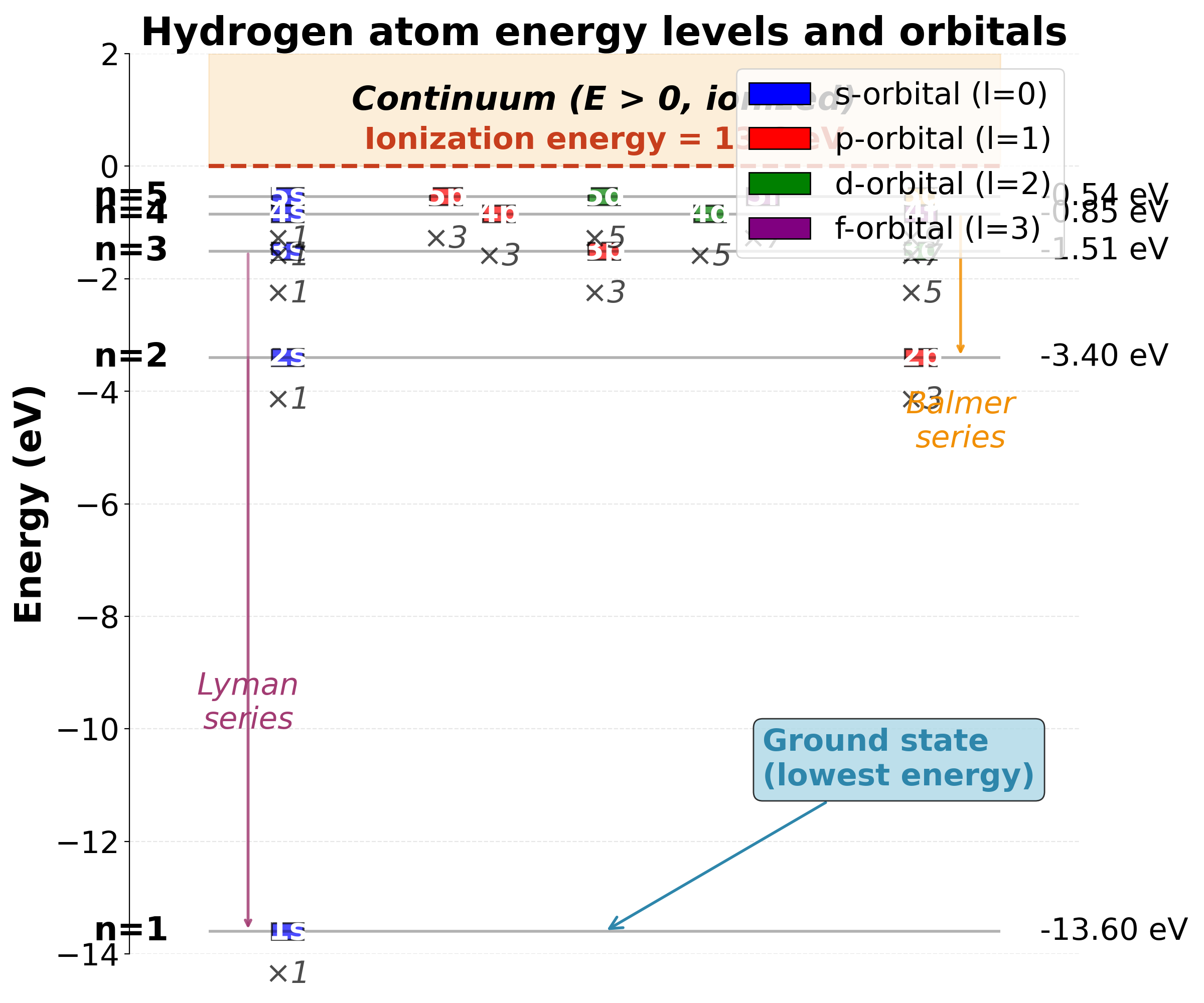
We observe attractive force between electron and nucleus. Solution: atomic orbitals with quantized energies.

Key insight: We see that the potential \(V(\mathbf{r})\) determines:
  • What regions the particle can access (classically forbidden if \(E < V\))

  • The shape of allowed wavefunctions

  • The quantized energy levels for bound states

  • The forces acting on the particle: \(\mathbf{F} = -\nabla V\)

Quantum tunneling: Unlike classical mechanics, we observe that particles can penetrate into regions where \(E < V\). We see that the wavefunction decays exponentially in these classically forbidden regions but doesn’t vanish completely.

Time-independent Schrödinger equation

When can we separate space and time?

For a time-independent potential \(V(\mathbf{r})\), we can write:

\[\psi(\mathbf{r}, t) = \psi(\mathbf{r}) e^{-iEt/\hbar}\]

where \(E\) is the energy. We find that the spatial part satisfies:

\[-\frac{\hbar^2}{2m} \nabla^2 \psi + V(\mathbf{r}) \psi = E \psi\]

This is what we call the time-independent Schrödinger equation (also called the energy eigenvalue equation).

Why does the time part have the form e^(-iEt/ℏ)?

We choose this form because it satisfies the time-dependent Schrödinger equation.

We start with the time-dependent Schrödinger equation:

\[i\hbar \frac{\partial \psi}{\partial t} = \hat{H} \psi\]

We try a solution \(\psi(\mathbf{r}, t) = \psi(\mathbf{r}) e^{-iEt/\hbar}\).

We take the time derivative:

\[\frac{\partial \psi}{\partial t} = \psi(\mathbf{r}) \frac{\partial}{\partial t}\left(e^{-iEt/\hbar}\right) = \psi(\mathbf{r}) \left(-\frac{iE}{\hbar}\right) e^{-iEt/\hbar} = -\frac{iE}{\hbar} \psi\]

We substitute into the Schrödinger equation:

\[i\hbar \left(-\frac{iE}{\hbar} \psi\right) = \hat{H} \psi\]
\[i\hbar \cdot \left(-\frac{iE}{\hbar}\right) \psi = E\psi = \hat{H} \psi\]

We see that this works! The time dependence \(e^{-iEt/\hbar}\) ensures the Schrödinger equation is satisfied when the Hamiltonian acting on the spatial part gives \(E\psi\).

Physical meaning: We observe that the phase rotates at frequency \(\omega = E/\hbar\). We see that higher energy gives faster rotation in the complex plane.

Separation of variables derivation

Start with the time-dependent Schrödinger equation:

\[i\hbar \frac{\partial \psi}{\partial t} = -\frac{\hbar^2}{2m} \nabla^2 \psi + V(\mathbf{r}) \psi\]

Assume the potential doesn’t depend on time: \(V = V(\mathbf{r})\). Try a solution of the form:

\[\psi(\mathbf{r}, t) = \psi(\mathbf{r}) T(t)\]

Substitute:

\[i\hbar \psi(\mathbf{r}) \frac{dT}{dt} = T(t) \left[-\frac{\hbar^2}{2m} \nabla^2 \psi + V(\mathbf{r}) \psi\right]\]

Divide both sides by \(\psi(\mathbf{r}) T(t)\):

\[i\hbar \frac{1}{T} \frac{dT}{dt} = \frac{1}{\psi} \left[-\frac{\hbar^2}{2m} \nabla^2 \psi + V(\mathbf{r}) \psi\right]\]

The left side depends only on \(t\), the right side only on \(\mathbf{r}\). Both must equal a constant, which we call \(E\):

\[i\hbar \frac{dT}{dt} = ET \quad \Rightarrow \quad T(t) = e^{-iEt/\hbar}\]
\[-\frac{\hbar^2}{2m} \nabla^2 \psi + V(\mathbf{r}) \psi = E \psi\]

This is the time-independent Schrödinger equation.

Free particle solutions

What is the wavefunction for a free electron?

For a free particle (\(V = 0\)), we see that the Schrödinger equation becomes:

\[-\frac{\hbar^2}{2m} \nabla^2 \psi = E \psi\]

We find that the solution is a plane wave:

\[\psi(\mathbf{r}, t) = A e^{i(\mathbf{k} \cdot \mathbf{r} - \omega t)}\]
where:
  • \(\mathbf{k}\): wave vector (direction of propagation)

  • \(|\mathbf{k}| = 2\pi/\lambda\): wave number

  • \(\omega = E/\hbar\): angular frequency

We obtain the dispersion relation:

\[E = \frac{\hbar^2 k^2}{2m} = \frac{p^2}{2m}\]

We see that this connects the wave picture (\(k\)) to the particle picture (\(p = \hbar k\)).

Wave packets and time evolution

The problem with plane waves

Why can’t a particle be a plane wave?

We just saw that free particle solutions are plane waves \(\psi = e^{i(kx - \omega t)}\). But we encounter a fundamental problem: plane waves are not normalizable!

\[\int_{-\infty}^{\infty} |e^{ikx}|^2 dx = \int_{-\infty}^{\infty} 1 \, dx = \infty\]

We see that a plane wave exists with equal probability everywhere in space (\(|\psi|^2 = 1\) at all \(x\)). We observe that this violates normalization and doesn’t represent a localized particle.

Physical problem:
  • We find that a plane wave has definite momentum \(p = \hbar k\) but completely undefined position (\(\Delta x = \infty\))

  • We see this is consistent with uncertainty (\(\Delta x \cdot \Delta p \geq \hbar/2\) with \(\Delta p = 0 \Rightarrow \Delta x = \infty\))

  • But we observe that real particles are localized somewhere!

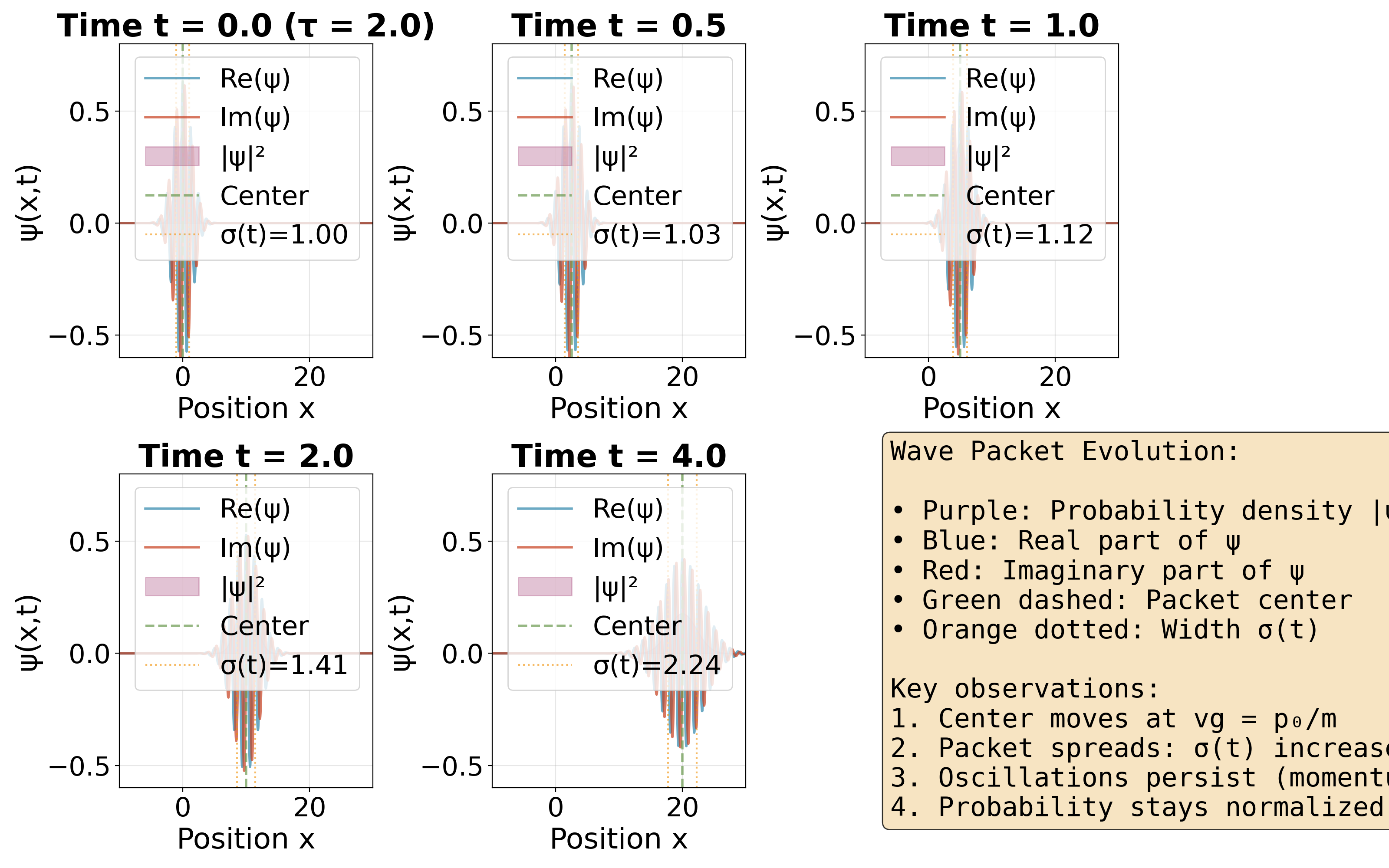
What is a wave packet?

We construct a wave packet as a superposition of plane waves with different momenta, built to be localized in space:

\[\psi(x,t) = \frac{1}{\sqrt{2\pi}} \int_{-\infty}^{\infty} A(k) e^{i(kx - \omega(k)t)} dk\]

Here, we have \(A(k)\) as the amplitude distribution in momentum space.

Key idea: We see that by combining waves with slightly different wavelengths (momenta), we create constructive interference in one region (localized particle) and destructive interference elsewhere.

Physical interpretation:
  • We find that \(|A(k)|^2\) gives the probability distribution in momentum space

  • We see that \(|\psi(x,t)|^2\) gives the probability distribution in position space

  • We observe that the packet represents a particle that is localized but not perfectly defined in position or momentum

Gaussian wave packets

The most common example
We see that the Gaussian wave packet is the most important example because:
  1. It minimizes the uncertainty principle (\(\Delta x \cdot \Delta p = \hbar/2\))

  2. It remains Gaussian under free time evolution (shape preserved)

  3. It’s analytically tractable

Initial wavefunction (at \(t=0\)):

\[\psi(x,0) = \left(\frac{1}{2\pi\sigma^2}\right)^{1/4} e^{ik_0 x} e^{-x^2/(4\sigma^2)}\]
Here, we have:
  • \(\sigma\): width of the packet (position uncertainty)

  • \(k_0\): central wave number (average momentum \(p_0 = \hbar k_0\))

  • \(e^{ik_0 x}\): plane wave carrier

  • \(e^{-x^2/(4\sigma^2)}\): Gaussian envelope

Momentum space representation:

\[A(k) = \left(\frac{2\sigma^2}{\pi}\right)^{1/4} e^{-\sigma^2(k-k_0)^2}\]

We observe that this is also Gaussian! We find that the packet is localized in both position and momentum space.

Uncertainties for Gaussian packets

For a Gaussian wave packet, we calculate:

\[\Delta x = \sigma, \quad \Delta p = \frac{\hbar}{2\sigma}\]
\[\boxed{\Delta x \cdot \Delta p = \frac{\hbar}{2}}\]

We see that this saturates the uncertainty bound – Gaussian packets are the most localized possible quantum states!

Trade-off:
  • We observe that narrow in position (\(\sigma\) small) gives wide in momentum (\(\Delta p\) large)

  • We find that narrow in momentum (\(\sigma\) large) gives wide in position (\(\Delta x\) large)

Time evolution of wave packets

How does a wave packet evolve?

For a free particle, we observe that each momentum component evolves with its own frequency \(\omega(k) = \hbar k^2/(2m)\):

\[\psi(x,t) = \frac{1}{\sqrt{2\pi}} \int_{-\infty}^{\infty} A(k) e^{i(kx - \omega(k)t)} dk\]

Key insight: We see that different frequency components travel at different speeds! We observe that this causes the packet to spread out over time.

Time evolution of Gaussian wave packets

For a Gaussian packet starting at \(x=0\) with width \(\sigma\), we find:

\[\psi(x,t) = \left(\frac{1}{2\pi\sigma(t)^2}\right)^{1/4} e^{ik_0(x - v_g t)} e^{-(x-v_g t)^2/(4\sigma(t)^2)}\]

Here, we have:

\[v_g = \frac{\hbar k_0}{m} = \frac{p_0}{m} \quad \text{(group velocity)}\]
\[\sigma(t) = \sigma \sqrt{1 + \left(\frac{\hbar t}{2m\sigma^2}\right)^2} \quad \text{(time-dependent width)}\]

Observations:

  1. Center moves classically: We see that \(x_{\text{center}}(t) = v_g t = p_0 t/m\) (Newton’s law!)

  2. Packet spreads: We observe that \(\sigma(t) > \sigma\) for all \(t > 0\)

  3. Spreading rate: We find faster spreading for narrow packets (small \(\sigma\)) and light particles (small \(m\))

Spreading of wave packets

Characteristic spreading time

We define the time scale for significant spreading:

\[\tau = \frac{2m\sigma^2}{\hbar}\]

We see that at time \(t = \tau\), the width has increased by \(\sqrt{2}\):

\[\sigma(\tau) = \sqrt{2} \, \sigma\]

For short times (\(t \ll \tau\)): We find that \(\sigma(t) \approx \sigma\) (minimal spreading)

For long times (\(t \gg \tau\)): We observe that \(\sigma(t) \approx \frac{\hbar t}{2m\sigma}\) (linear spreading)

Physical examples of spreading

Electron in an atom (\(\sigma \sim 10^{-10}\) m, \(m = 9.1 \times 10^{-31}\) kg):

\[\tau = \frac{2m\sigma^2}{\hbar} \sim 10^{-16} \text{ s}\]

We see that it spreads incredibly fast! This is why we describe electrons in atoms using stationary states, not localized packets.

Macroscopic object (dust particle: \(\sigma \sim 10^{-6}\) m, \(m \sim 10^{-15}\) kg):

\[\tau \sim 10^{9} \text{ years}\]

We observe that it effectively never spreads during experimental timescales. This is why we don’t see quantum spreading in everyday life!

Key principle: We have \(\tau \propto m\sigma^2/\hbar\). We see that heavier and larger objects spread much more slowly.

Group velocity vs phase velocity

Two important velocities

For a wave packet, we distinguish two velocities:

Phase velocity: We define the speed at which a single wave crest moves:

\[v_{\text{phase}} = \frac{\omega}{k} = \frac{\hbar k}{2m}\]

Group velocity: We calculate the speed at which the packet envelope (the “particle”) moves:

\[v_{\text{group}} = \frac{d\omega}{dk} = \frac{\hbar k}{m}\]

Key observation: We see that \(v_{\text{group}} = 2 v_{\text{phase}}\) for matter waves!

Physical meaning:
  • We observe that individual wave crests move at \(v_{\text{phase}}\)

  • We find that the packet center (observable particle) moves at \(v_{\text{group}} = p/m\) (classical velocity!)

  • We see that wave crests appear at the back of the packet, move through it, and disappear at the front

Why group velocity matters

We measure the group velocity as what we actually observe as the particle’s velocity:

\[v_g = \frac{d\omega}{dk} = \frac{d}{dk}\left(\frac{\hbar k^2}{2m}\right) = \frac{\hbar k}{m} = \frac{p}{m}\]

We see that this matches the classical momentum-velocity relation! We observe that quantum mechanics reproduces classical motion for the center of wave packets.

Dispersion

What is dispersion?

We observe that dispersion occurs when the relationship \(\omega(k)\) is nonlinear. For quantum particles:

\[\omega(k) = \frac{\hbar k^2}{2m}\]

We see that this is quadratic (not linear), causing different frequency components to travel at different speeds.

Consequence: We find that the packet spreads because high-momentum components (large \(k\)) travel faster than low-momentum components.

Dispersion relation determines spreading

We observe that the spreading rate depends on the curvature of \(\omega(k)\):

\[\frac{d^2\omega}{dk^2} = \frac{\hbar}{m}\]
Larger curvature means faster spreading. For quantum particles:
  • We see that light particles (small \(m\)) spread faster

  • We find that heavy particles (large \(m\)) spread slower

Photons (\(\omega = ck\), linear!) don’t spread at all in vacuum. But we observe that quantum particles (\(\omega \propto k^2\)) always spread.

Visualization: Wave packet dynamics

Let me create a comprehensive visualization showing wave packet evolution:

(Source code, png, hires.png, pdf)

../_images/quantum-1-1.png

The figure above shows a Gaussian wave packet evolving over time. Notice how:

  1. The center moves: Position \(x_{\text{center}} = v_g t\) increases linearly (green dashed line)

  2. The packet spreads: Width \(\sigma(t)\) increases (orange dotted lines move apart)

  3. Oscillations remain: The wave structure (blue/red curves) persists but spreads out

  4. Probability is conserved: Total area under purple curve stays constant

Momentum space representation

The complementary picture

We can also visualize the wave packet in momentum space by taking the Fourier transform:

\[A(k) = \frac{1}{\sqrt{2\pi}} \int_{-\infty}^{\infty} \psi(x,0) e^{-ikx} dx\]

For a Gaussian wave packet:

\[|A(k)|^2 = \frac{2\sigma}{\sqrt{\pi}} e^{-2\sigma^2(k-k_0)^2}\]

Key insight: As the position-space packet spreads (\(\sigma(t)\) increases), the momentum-space width stays constant!

Physical meaning: Spreading doesn’t change the momentum distribution – it’s determined by the initial conditions. The packet spreads because different momenta correspond to different velocities.

(Source code, png, hires.png, pdf)

../_images/quantum-1-2.png

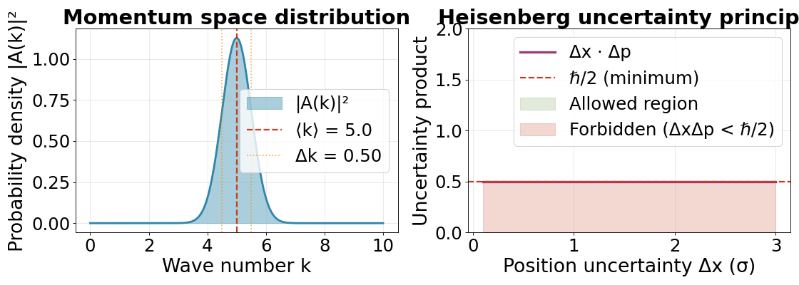
Left panel: We see that the momentum distribution \(|A(k)|^2\) is Gaussian, centered at \(k_0\) with width \(\Delta k = 1/(2\sigma)\). We observe that this distribution doesn’t change as the packet spreads!

Right panel: We find the uncertainty product \(\Delta x \cdot \Delta p\) for Gaussian packets. We see that the minimum value \(\hbar/2\) (red line) is achieved, making Gaussians the most localized possible states.

Why wave packets matter

Wave packets bridge quantum and classical physics

1. Localization: Unlike plane waves, we see that packets represent localized particles

2. Classical limit: We observe that packet center moves according to \(F = ma\)

3. Uncertainty principle: We find that \(\Delta x \cdot \Delta p \geq \hbar/2\) is manifest

4. Quantum spreading: We see deviations from classical behavior (spreading)

5. Real experiments: We observe that actual quantum states are wave packets, not energy eigenstates

Applications of wave packet physics

Femtosecond chemistry: We see that ultra-short laser pulses create wave packets that probe molecular dynamics

Atom interferometry: We observe that wave packets of atoms interfere to measure gravity and fundamental constants

Quantum computing: We find that qubit manipulations create and evolve wave packets in Hilbert space

Particle physics: We see that relativistic wave packets describe particle propagation

Summary: Key insights from wave packets

Property

Gaussian wave packet

Position uncertainty

\(\Delta x = \sigma(t) = \sigma\sqrt{1 + (\hbar t/(2m\sigma^2))^2}\)

Momentum uncertainty

\(\Delta p = \hbar/(2\sigma)\) (constant in time)

Uncertainty product

\(\Delta x \cdot \Delta p = \hbar/2\) (minimum possible)

Center position

\(x_c(t) = p_0 t/m\) (classical motion)

Spreading time

\(\tau = 2m\sigma^2/\hbar\)

Group velocity

\(v_g = p_0/m = \hbar k_0/m\)

Long-time behavior

\(\sigma(t) \approx \hbar t/(2m\sigma)\) for \(t \gg \tau\)

The hydrogen atom

Why is the hydrogen atom so important?

The hydrogen atom is the most important problem in quantum mechanics for several reasons:

1. Exactly solvable: One of the few quantum systems we can solve analytically (unlike multi-electron atoms)

2. Fundamental physics: Understanding how electrons bind to nuclei explains all of chemistry

3. Spectroscopy: Predicted energy levels match experimental spectral lines with incredible precision

4. Historical significance: First triumph of quantum mechanics, explaining the mysterious Balmer series

5. Universal patterns: The quantum numbers (\(n, l, m\)) and orbital structure appear throughout physics

Every atom in the periodic table builds on hydrogen’s quantum structure. Master this, and we understand the foundation of atomic physics!

The Coulomb potential

Setting up the problem

A hydrogen atom has one electron (charge \(-e\)) bound to one proton (charge \(+e\)). The electrostatic potential energy is:

\[V(r) = -\frac{e^2}{4\pi\epsilon_0 r} = -\frac{ke^2}{r}\]

where \(r\) is the distance between electron and proton, and \(k = 1/(4\pi\epsilon_0) \approx 9 \times 10^9\) N·m²/C².

Key features:
  • \(V(r) \to 0\) as \(r \to \infty\) (free electron reference)

  • \(V(r) \to -\infty\) as \(r \to 0\) (strong attraction at nucleus)

  • Spherically symmetric: \(V\) depends only on \(r = |\vec{r}|\), not on direction

Simplification: Treat the nucleus as infinitely heavy (fixed at origin). More accurately, use the reduced mass \(\mu = m_e m_p/(m_e + m_p) \approx m_e\).

The time-independent Schrödinger equation

For a stationary state with energy \(E\):

\[-\frac{\hbar^2}{2m_e}\nabla^2\psi - \frac{ke^2}{r}\psi = E\psi\]

In Cartesian coordinates, \(\nabla^2 = \partial^2/\partial x^2 + \partial^2/\partial y^2 + \partial^2/\partial z^2\). But this is a nightmare to solve!

Key insight: The potential has spherical symmetry, so use spherical coordinates \((r, \theta, \phi)\).

Separation of variables in spherical coordinates

Why spherical coordinates?

When the potential depends only on \(r\), spherical coordinates \((r, \theta, \phi)\) are natural:

\[x = r\sin\theta\cos\phi, \quad y = r\sin\theta\sin\phi, \quad z = r\cos\theta\]

The Laplacian becomes:

\[\nabla^2 = \frac{1}{r^2}\frac{\partial}{\partial r}\left(r^2\frac{\partial}{\partial r}\right) + \frac{1}{r^2\sin\theta}\frac{\partial}{\partial\theta}\left(\sin\theta\frac{\partial}{\partial\theta}\right) + \frac{1}{r^2\sin^2\theta}\frac{\partial^2}{\partial\phi^2}\]

This looks complicated, but it allows separation of variables!

Assuming a separable solution

Try a solution of the form:

\[\psi(r,\theta,\phi) = R(r) Y(\theta,\phi)\]

where \(R(r)\) is the radial function and \(Y(\theta,\phi)\) is the angular function.

Physical meaning:
  • \(R(r)\): How far the electron is from the nucleus

  • \(Y(\theta,\phi)\): Which direction the electron is likely to be found

Substituting into the Schrödinger equation and dividing by \(R(r)Y(\theta,\phi)\):

\[\frac{1}{R}\frac{d}{dr}\left(r^2\frac{dR}{dr}\right) - \frac{2m_e r^2}{\hbar^2}\left(V(r) - E\right) = -\frac{1}{Y}\left[\frac{1}{\sin\theta}\frac{\partial}{\partial\theta}\left(\sin\theta\frac{\partial Y}{\partial\theta}\right) + \frac{1}{\sin^2\theta}\frac{\partial^2 Y}{\partial\phi^2}\right]\]

Key observation: Left side depends only on \(r\), right side only on \((\theta,\phi)\). Both must equal a constant!

The angular equation and spherical harmonics

Separation constant and angular momentum

The separation constant turns out to be \(l(l+1)\), where \(l\) is an integer. This gives:

\[\frac{1}{\sin\theta}\frac{\partial}{\partial\theta}\left(\sin\theta\frac{\partial Y}{\partial\theta}\right) + \frac{1}{\sin^2\theta}\frac{\partial^2 Y}{\partial\phi^2} = -l(l+1)Y\]

This is the angular momentum eigenvalue equation! The solutions are spherical harmonics \(Y_l^m(\theta,\phi)\).

Spherical harmonics: \(Y_l^m(\theta,\phi)\)

The angular solutions are labeled by two quantum numbers:

Orbital angular momentum quantum number \(l\):
  • \(l = 0, 1, 2, 3, \ldots\)

  • Determines the magnitude of angular momentum: \(L = \hbar\sqrt{l(l+1)}\)

  • Historical notation: \(l=0\) (s), \(l=1\) (p), \(l=2\) (d), \(l=3\) (f), …

Magnetic quantum number \(m\):
  • \(m = -l, -l+1, \ldots, 0, \ldots, l-1, l\)

  • Determines the \(z\)-component of angular momentum: \(L_z = m\hbar\)

  • For each \(l\), there are \(2l+1\) possible values of \(m\)

First few spherical harmonics
\[Y_0^0 &= \frac{1}{\sqrt{4\pi}} \quad \text{(s orbital: spherically symmetric)}\]
\[Y_1^0 &= \sqrt{\frac{3}{4\pi}}\cos\theta \quad \text{(pz orbital)}\]
\[Y_1^{\pm 1} &= \mp\sqrt{\frac{3}{8\pi}}\sin\theta \, e^{\pm i\phi} \quad \text{(px, py orbitals)}\]
\[Y_2^0 &= \sqrt{\frac{5}{16\pi}}(3\cos^2\theta - 1) \quad \text{(dz² orbital)}\]

Key property: Spherical harmonics are orthonormal:

\[\int_0^{2\pi}\int_0^\pi Y_l^m(\theta,\phi)^* Y_{l'}^{m'}(\theta,\phi) \sin\theta \, d\theta \, d\phi = \delta_{ll'}\delta_{mm'}\]

The radial equation

After separating angular part

With \(Y(\theta,\phi) = Y_l^m(\theta,\phi)\), the radial equation becomes:

\[-\frac{\hbar^2}{2m_e}\frac{1}{r^2}\frac{d}{dr}\left(r^2\frac{dR}{dr}\right) + \left[\frac{\hbar^2 l(l+1)}{2m_e r^2} - \frac{ke^2}{r}\right]R = ER\]

Effective potential:

\[V_{\text{eff}}(r) = \frac{\hbar^2 l(l+1)}{2m_e r^2} - \frac{ke^2}{r}\]
This has two terms:
  • \(\hbar^2 l(l+1)/(2m_e r^2)\): Centrifugal barrier (repulsive, keeps electron away from nucleus for \(l > 0\))

  • \(-ke^2/r\): Coulomb attraction

Substitution to simplify

Define \(u(r) = r R(r)\). Then:

\[-\frac{\hbar^2}{2m_e}\frac{d^2u}{dr^2} + \left[\frac{\hbar^2 l(l+1)}{2m_e r^2} - \frac{ke^2}{r}\right]u = Eu\]

This looks like a 1D Schrödinger equation with effective potential \(V_{\text{eff}}(r)\)!

Boundary conditions:
  • \(u(0) = 0\) (wavefunction finite at origin)

  • \(u(\infty) = 0\) (bound state, normalizable)

Energy quantization: The principal quantum number

Solving the radial equation

The radial equation can be solved using power series methods (Frobenius method). The requirement that \(u(r) \to 0\) as \(r \to \infty\) quantizes the energy!

Result: Bound states exist only for discrete energies:

\[\boxed{E_n = -\frac{m_e k^2 e^4}{2\hbar^2 n^2} = -\frac{13.6 \text{ eV}}{n^2}}\]

where \(n = 1, 2, 3, \ldots\) is the principal quantum number.

The Bohr radius

Define the Bohr radius:

\[a_0 = \frac{\hbar^2}{m_e k e^2} = 0.529 \text{ Å}\]

This is the characteristic size of the hydrogen atom! Then:

\[E_n = -\frac{\hbar^2}{2m_e a_0^2 n^2} = -\frac{13.6 \text{ eV}}{n^2}\]

Physical interpretation: \(a_0\) is roughly the radius of the ground state orbit.

Quantum number constraints

The three quantum numbers must satisfy:

\[n = 1, 2, 3, \ldots\]
\[l = 0, 1, 2, \ldots, n-1 \quad \text{(for each } n\text{)}\]
\[m = -l, -l+1, \ldots, 0, \ldots, l-1, l \quad \text{(for each } l\text{)}\]

Key constraint: \(l < n\). The orbital angular momentum is limited by the energy level!

Degeneracy: For a given \(n\), the number of states is:

\[\sum_{l=0}^{n-1}(2l+1) = n^2\]

All these \(n^2\) states have the same energy \(E_n\) (before spin)!

Hydrogen atom energy levels

The energy level diagram

(Source code)

Key observations from the diagram:

  1. Energy depends only on n: We see that all orbitals with the same \(n\) have the same energy (degeneracy)

  2. Energy spacing: We observe that levels get closer together as \(n\) increases (\(E_n \propto 1/n^2\))

  3. Subshells: We find that each \(n\) contains \(n\) different \(l\) values (1s, 2s 2p, 3s 3p 3d, etc.)

  4. Degeneracy: We see that the \(\times\text{number}\) shows how many \(m\) states each sublevel has

  5. Spectral lines: We observe that transitions between levels produce photons (Lyman, Balmer series)

  6. Ionization: We see that \(E = 0\) separates bound states (negative energy) from free electrons

Radial wavefunctions

General form

We find that the radial functions \(R_{nl}(r)\) have the form:

\[R_{nl}(r) = N_{nl} \left(\frac{r}{a_0}\right)^l e^{-r/(na_0)} L_{n-l-1}^{2l+1}\left(\frac{2r}{na_0}\right)\]

where \(L_{n-l-1}^{2l+1}\) are associated Laguerre polynomials and \(N_{nl}\) is a normalization constant.

Don’t worry about the details! We observe the key features:
  • Factor \(r^l\): We see that this keeps electron away from nucleus for \(l > 0\) (centrifugal barrier)

  • Exponential \(e^{-r/(na_0)}\): We find that this creates decay at large \(r\)

  • Polynomial: We observe that this creates nodes (radial nodes = \(n - l - 1\))

First few radial functions

Ground state (\(n=1, l=0\)):

\[R_{10}(r) = 2\left(\frac{1}{a_0}\right)^{3/2} e^{-r/a_0}\]

First excited states (\(n=2\)):

\[R_{20}(r) = \frac{1}{2\sqrt{2}}\left(\frac{1}{a_0}\right)^{3/2}\left(2 - \frac{r}{a_0}\right)e^{-r/(2a_0)}\]
\[R_{21}(r) = \frac{1}{2\sqrt{6}}\left(\frac{1}{a_0}\right)^{3/2}\frac{r}{a_0}e^{-r/(2a_0)}\]
Radial probability density

We calculate the probability of finding the electron at distance \(r\) (in a thin shell) as:

\[P(r) = 4\pi r^2 |R_{nl}(r)|^2\]

We see that the factor \(4\pi r^2\) is the surface area of a sphere, meaning there’s more “room” at larger \(r\)!

(Source code)

Key observations from radial plots:

  1. Radial nodes: Number of nodes = \(n - l - 1\) (where \(R_{nl} = 0\)) - 1s has 0 nodes, 2s has 1 node, 3s has 2 nodes, etc.

  2. Most probable radius: Peak of \(P(r)\) (red) shows where electron is most likely found - For 1s: \(r_{\text{max}} = a_0\) (the Bohr radius!) - Generally increases with \(n\) (higher energy → larger orbit)

  3. Centrifugal barrier: Higher \(l\) → electron pushed away from nucleus (\(R \propto r^l\) near origin)

  4. Exponential decay: All states decay as \(e^{-r/(na_0)}\) at large \(r\)

Complete hydrogen atom wavefunctions

The full wavefunction

The complete solution combines radial and angular parts:

\[\boxed{\psi_{nlm}(r,\theta,\phi) = R_{nl}(r) Y_l^m(\theta,\phi)}\]
Three quantum numbers:
  • \(n\): Principal (energy, size)

  • \(l\): Orbital angular momentum (shape)

  • \(m\): Magnetic (orientation in space)

Normalization

The wavefunctions are normalized over all space:

\[\int_0^{\infty}\int_0^{\pi}\int_0^{2\pi} |\psi_{nlm}|^2 r^2\sin\theta \, dr\,d\theta\,d\phi = 1\]

This can be split:

\[\int_0^{\infty} |R_{nl}(r)|^2 r^2 dr = 1, \quad \int_0^{\pi}\int_0^{2\pi} |Y_l^m(\theta,\phi)|^2 \sin\theta \, d\theta\,d\phi = 1\]
Orthogonality

Different states are orthogonal:

\[\langle \psi_{nlm} | \psi_{n'l'm'} \rangle = \delta_{nn'}\delta_{ll'}\delta_{mm'}\]

This is crucial for: measurement theory, perturbation theory, selection rules.

Visualizing hydrogen orbitals

Let me create comprehensive orbital visualizations:

import numpy as np
import matplotlib.pyplot as plt
from mpl_toolkits.mplot3d import Axes3D
from scipy.special import sph_harm

# Define spherical harmonics squared (probability densities)
def Y_00(theta, phi):
    return np.ones_like(theta) / np.sqrt(4*np.pi)

def Y_10(theta, phi):
    return np.sqrt(3/(4*np.pi)) * np.cos(theta)

def Y_1m1(theta, phi):
    return np.sqrt(3/(8*np.pi)) * np.sin(theta) * np.exp(-1j*phi)

def Y_1p1(theta, phi):
    return -np.sqrt(3/(8*np.pi)) * np.sin(theta) * np.exp(1j*phi)

def Y_20(theta, phi):
    return np.sqrt(5/(16*np.pi)) * (3*np.cos(theta)**2 - 1)

fig = plt.figure(figsize=(16, 12))

# Create grid in spherical coordinates
theta = np.linspace(0, np.pi, 100)
phi = np.linspace(0, 2*np.pi, 100)
theta_grid, phi_grid = np.meshgrid(theta, phi)

# Orbital data: (Y_func, title, subplot_pos)
orbitals = [
    (Y_00, '1s (l=0, m=0)', 1),
    (Y_10, '2pz (l=1, m=0)', 2),
    (lambda t, p: Y_1m1(t, p) - Y_1p1(t, p), '2px (l=1, mx)', 3),
    (lambda t, p: 1j*(Y_1m1(t, p) + Y_1p1(t, p)), '2py (l=1, my)', 4),
    (Y_20, '3dz² (l=2, m=0)', 5),
]

for Y_func, title, pos in orbitals:
    ax = fig.add_subplot(2, 3, pos, projection='3d')

    # Calculate angular function
    Y = Y_func(theta_grid, phi_grid)
    Y_abs = np.abs(Y)

    # Normalize for visualization
    Y_abs_norm = Y_abs / Y_abs.max()

    # Convert to Cartesian (radius determined by |Y|²)
    r = Y_abs_norm
    x = r * np.sin(theta_grid) * np.cos(phi_grid)
    y = r * np.sin(theta_grid) * np.sin(phi_grid)
    z = r * np.cos(theta_grid)

    # Color by sign of real part
    colors = np.real(Y)

    # Plot surface
    surf = ax.plot_surface(x, y, z, facecolors=plt.cm.seismic(colors/colors.max()),
                          alpha=0.8, linewidth=0, antialiased=True, shade=True)

    # Formatting
    ax.set_xlabel('x', fontsize=24)
    ax.set_ylabel('y', fontsize=24)
    ax.set_zlabel('z', fontsize=24)
    ax.set_title(title, fontsize=26, weight='bold')
    ax.tick_params(axis='both', labelsize=22)

    # Set equal aspect ratio
    max_range = 1.0
    ax.set_xlim([-max_range, max_range])
    ax.set_ylim([-max_range, max_range])
    ax.set_zlim([-max_range, max_range])
    ax.set_box_aspect([1,1,1])

# Add explanation panel
ax = fig.add_subplot(2, 3, 6)
ax.axis('off')
text = (
    "Orbital visualization notes:\n\n"
    "• Surface shows |Y(θ,φ)|²\n"
    "• Color: blue (+), red (−) phase\n"
    "• s orbitals: spherical\n"
    "• p orbitals: dumbbell shape\n"
    "• d orbitals: complex lobes\n\n"
    "Quantum numbers:\n"
    "• l = 0: s (1 orbital)\n"
    "• l = 1: p (3 orbitals)\n"
    "• l = 2: d (5 orbitals)\n"
    "• l = 3: f (7 orbitals)\n\n"
    "Each n contains orbitals\n"
    "for l = 0, 1, ..., n−1"
)
ax.text(0.1, 0.5, text, fontsize=22, family='monospace',
       verticalalignment='center', bbox=dict(boxstyle='round',
       facecolor='lightyellow', alpha=0.9))

plt.tight_layout()

(Source code)

Understanding orbital shapes:

  1. s orbitals (\(l=0\)): Spherically symmetric, no angular dependence

  2. p orbitals (\(l=1\)): Dumbbell-shaped, three orientations (px, py, pz) - \(p_z\) points along z-axis - \(p_x, p_y\) point along x, y axes (linear combinations of \(m = \pm 1\))

  3. d orbitals (\(l=2\)): More complex lobes, five orientations - \(d_{z^2}\): Special shape along z-axis - \(d_{xy}, d_{xz}, d_{yz}, d_{x^2-y^2}\): Four-lobed patterns

  4. Phase/sign: Color indicates sign of wavefunction (important for bonding!)

Spectroscopy and transitions

Photon emission and absorption

When an electron transitions between energy levels:

\[\Delta E = E_{n_f} - E_{n_i} = h\nu = \frac{hc}{\lambda}\]

where \(\nu\) is photon frequency and \(\lambda\) is wavelength.

Emission: Electron drops from high \(n\) to low \(n\), emits photon

Absorption: Electron jumps from low \(n\) to high \(n\), absorbs photon

The hydrogen spectrum

Lyman series (\(n \to 1\)): UV photons

\[\lambda = \frac{hc}{13.6 \text{ eV}} \frac{n^2}{n^2 - 1} \quad (n = 2, 3, 4, \ldots)\]

Balmer series (\(n \to 2\)): Visible light! This is what Balmer discovered empirically in 1885.

\[\lambda = \frac{hc}{13.6 \text{ eV}} \frac{4n^2}{n^2 - 4} \quad (n = 3, 4, 5, \ldots)\]

Paschen series (\(n \to 3\)): Infrared

Selection rules

Not all transitions are allowed! Selection rules from angular momentum conservation:

\[\Delta l = \pm 1, \quad \Delta m = 0, \pm 1\]

Physical reason: A photon carries angular momentum \(L_{\gamma} = \hbar\), so \(l\) must change by 1.

Examples:
  • \(1s \to 2p\): Allowed (\(\Delta l = 1\))

  • \(1s \to 2s\): Forbidden (\(\Delta l = 0\))

  • \(2p \to 3d\): Allowed (\(\Delta l = 1\))

Beyond hydrogen: Multi-electron atoms

What changes with more electrons?

For atoms with \(Z > 1\) (helium, lithium, etc.):

1. Electron-electron repulsion: Electrons repel each other, breaking the simple \(-Ze^2/r\) potential

2. Screening: Inner electrons “shield” the nuclear charge from outer electrons

3. Energy splitting: Orbitals with the same \(n\) but different \(l\) no longer have the same energy!
  • Example: In multi-electron atoms, 3d has higher energy than 3s or 3p

  • Ordering: \(E_{ns} < E_{np} < E_{nd} < E_{nf}\)

4. Pauli exclusion: No two electrons can have identical quantum numbers (needs spin!)

5. Aufbau principle: Electrons fill orbitals from lowest to highest energy

But the quantum numbers \((n, l, m)\) and orbital shapes from hydrogen remain valid! This is why the periodic table has the structure it does.

Summary: The hydrogen atom

Concept

Key result

Potential

\(V(r) = -ke^2/r\) (Coulomb attraction)

Energy levels

\(E_n = -13.6 \text{ eV}/n^2\) (quantized!)

Bohr radius

\(a_0 = \hbar^2/(m_e ke^2) = 0.529\) Å

Quantum numbers

\(n = 1, 2, 3, \ldots\); \(l = 0, \ldots, n-1\); \(m = -l, \ldots, l\)

Degeneracy

\(n^2\) states per energy level

Wavefunction

\(\psi_{nlm} = R_{nl}(r) Y_l^m(\theta,\phi)\)

Angular momentum

\(L = \hbar\sqrt{l(l+1)}\); \(L_z = m\hbar\)

Selection rules

\(\Delta l = \pm 1\); \(\Delta m = 0, \pm 1\)

Spectral series

Lyman (UV), Balmer (visible), Paschen (IR)

Angular momentum in quantum mechanics

Why is angular momentum so important?

Angular momentum is one of the most fundamental concepts in quantum mechanics because:

1. Conservation law: Angular momentum is conserved in isolated systems (from rotational symmetry)

2. Universal structure: The mathematics of angular momentum applies to every quantum system with rotation

3. Explains atomic structure: Orbital shapes, spectroscopy, and selection rules all come from angular momentum

4. Spin: Intrinsic angular momentum (spin) is purely quantum mechanical with no classical analog

5. Quantum numbers: The labels \(l, m\) that organize atomic orbitals come from angular momentum theory

Understanding angular momentum gives us a powerful framework that extends far beyond atoms to nuclei, molecules, and even elementary particles!

Classical angular momentum: A quick review

Classical definition

For a particle with position \(\vec{r}\) and momentum \(\vec{p}\), the angular momentum is:

\[\vec{L} = \vec{r} \times \vec{p}\]

In Cartesian components:

\[L_x = y p_z - z p_y, \quad L_y = z p_x - x p_z, \quad L_z = x p_y - y p_x\]
Key properties:
  • \(\vec{L}\) is perpendicular to both \(\vec{r}\) and \(\vec{p}\)

  • \(|\vec{L}|\) measures the “amount of rotation”

  • Direction gives the rotation axis (right-hand rule)

Conservation

If no external torque acts on a system, angular momentum is conserved:

\[\frac{d\vec{L}}{dt} = \vec{\tau}_{\text{external}}\]

This is Noether’s theorem in action: rotational symmetry → angular momentum conservation.

Quantum angular momentum operators

From classical to quantum

In quantum mechanics, we promote classical observables to operators by replacing:

\[x \to \hat{x}, \quad p_x \to \hat{p}_x = -i\hbar\frac{\partial}{\partial x}\]

The angular momentum operators become:

\[\hat{L}_x = \hat{y}\hat{p}_z - \hat{z}\hat{p}_y = -i\hbar\left(y\frac{\partial}{\partial z} - z\frac{\partial}{\partial y}\right)\]
\[\hat{L}_y = \hat{z}\hat{p}_x - \hat{x}\hat{p}_z = -i\hbar\left(z\frac{\partial}{\partial x} - x\frac{\partial}{\partial z}\right)\]
\[\hat{L}_z = \hat{x}\hat{p}_y - \hat{y}\hat{p}_x = -i\hbar\left(x\frac{\partial}{\partial y} - y\frac{\partial}{\partial x}\right)\]
Spherical coordinates

In spherical coordinates \((r, \theta, \phi)\), these simplify dramatically:

\[\hat{L}_z = -i\hbar\frac{\partial}{\partial\phi}\]
\[\hat{L}^2 = -\hbar^2\left[\frac{1}{\sin\theta}\frac{\partial}{\partial\theta}\left(\sin\theta\frac{\partial}{\partial\theta}\right) + \frac{1}{\sin^2\theta}\frac{\partial^2}{\partial\phi^2}\right]\]

This is why spherical coordinates are so useful! The angular momentum operators have simple forms.

Commutation relations: The heart of quantum angular momentum

The fundamental commutators

The key to understanding quantum angular momentum is the commutation relations:

\[[\hat{L}_x, \hat{L}_y] = i\hbar\hat{L}_z\]
\[[\hat{L}_y, \hat{L}_z] = i\hbar\hat{L}_x\]
\[[\hat{L}_z, \hat{L}_x] = i\hbar\hat{L}_y\]

Or compactly: \([\hat{L}_i, \hat{L}_j] = i\hbar\epsilon_{ijk}\hat{L}_k\) (where \(\epsilon_{ijk}\) is the Levi-Civita symbol).

What do these commutators mean?

Physical interpretation: You cannot simultaneously measure two different components of angular momentum!

\[\Delta L_x \cdot \Delta L_y \geq \frac{\hbar}{2}|\langle L_z \rangle|\]

Just like position-momentum uncertainty, but now for angular momentum components.

Example: If you measure \(L_z\) precisely (\(\Delta L_z = 0\)), then \(L_x\) and \(L_y\) become completely uncertain.

The total angular momentum operator

Define the total angular momentum squared:

\[\hat{L}^2 = \hat{L}_x^2 + \hat{L}_y^2 + \hat{L}_z^2\]

Key observation: \(\hat{L}^2\) commutes with each component!

\[[\hat{L}^2, \hat{L}_x] = [\hat{L}^2, \hat{L}_y] = [\hat{L}^2, \hat{L}_z] = 0\]

Physical meaning: We can simultaneously measure the total angular momentum magnitude and one component (conventionally \(L_z\)).

Eigenvalues and eigenstates of angular momentum

The eigenvalue problem

We want to find simultaneous eigenstates of \(\hat{L}^2\) and \(\hat{L}_z\):

\[\hat{L}^2 |l, m\rangle = \lambda |l, m\rangle\]
\[\hat{L}_z |l, m\rangle = \mu |l, m\rangle\]

The question is: What are the allowed values \(\lambda\) and \(\mu\)?

The answer from algebra alone

Using only the commutation relations (no differential equations!), we can prove:

\[\boxed{\lambda = \hbar^2 l(l+1), \quad l = 0, \frac{1}{2}, 1, \frac{3}{2}, 2, \ldots}\]
\[\boxed{\mu = \hbar m, \quad m = -l, -l+1, \ldots, l-1, l}\]

Key results:

  1. Total angular momentum: \(L^2\) has eigenvalues \(\hbar^2 l(l+1)\), not \(\hbar^2 l^2\)!

  2. Quantization: The quantum number \(l\) can be integer or half-integer (0, 1/2, 1, 3/2, 2, …)

  3. z-component: \(L_z = m\hbar\) where \(m\) ranges from \(-l\) to \(+l\) in integer steps

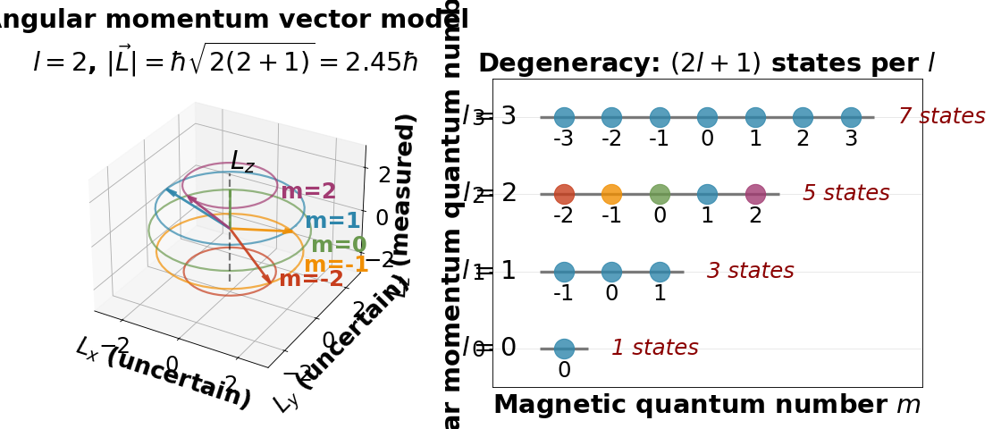
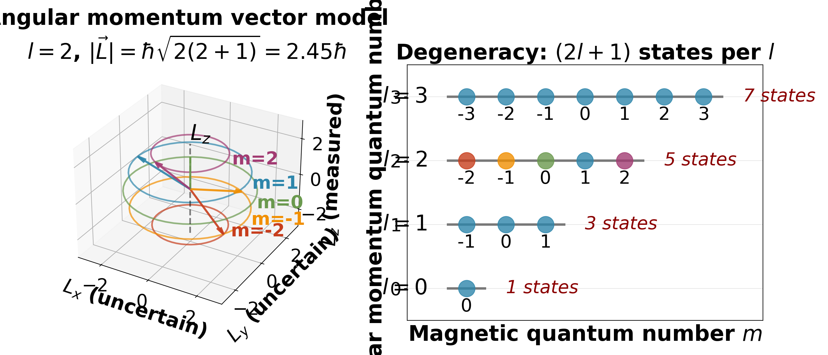
  4. Degeneracy: For each \(l\), there are \(2l+1\) possible values of \(m\)

Why \(l(l+1)\) and not \(l^2\)?

The magnitude of angular momentum is:

\[|\vec{L}| = \hbar\sqrt{l(l+1)}\]

This is always larger than \(|L_z|_{\max} = \hbar l\). Why?

Because \(L_x\) and \(L_y\) are uncertain! The angular momentum vector cannot point exactly along the z-axis. It “precesses” around the z-axis with uncertain \(x\) and \(y\) components.

import numpy as np
import matplotlib.pyplot as plt
from mpl_toolkits.mplot3d import Axes3D

fig = plt.figure(figsize=(14, 6))

# Left panel: Vector model for l=2
ax1 = fig.add_subplot(121, projection='3d')
l = 2
L_magnitude = np.sqrt(l*(l+1))

# Standard color palette for m quantum numbers
standard_colors = ['#C73E1D', '#F18F01', '#6A994E', '#2E86AB', '#A23B72']
colors_map = standard_colors[:2*l+1] if 2*l+1 <= len(standard_colors) else plt.cm.viridis(np.linspace(0, 1, 2*l+1))

for i, m in enumerate(range(-l, l+1)):
    L_z = m
    # L must have magnitude sqrt(l(l+1)), with z-component = m
    # So L_perp = sqrt(l(l+1) - m^2)
    L_perp = np.sqrt(L_magnitude**2 - L_z**2)

    # Draw cone at this L_z
    theta_cone = np.linspace(0, 2*np.pi, 50)
    x_cone = L_perp * np.cos(theta_cone)
    y_cone = L_perp * np.sin(theta_cone)
    z_cone = np.full_like(theta_cone, L_z)

    ax1.plot(x_cone, y_cone, z_cone, color=colors_map[i], linewidth=2, alpha=0.7)

    # Draw one example vector
    angle = i * np.pi / 3
    x_vec = L_perp * np.cos(angle)
    y_vec = L_perp * np.sin(angle)
    ax1.quiver(0, 0, 0, x_vec, y_vec, L_z, color=colors_map[i],
              arrow_length_ratio=0.15, linewidth=2.5, alpha=0.9)

    # Label m value
    label_r = L_perp + 0.3
    ax1.text(label_r, 0, L_z, f'm={m}', fontsize=22, weight='bold', color=colors_map[i])

# Draw z-axis
ax1.plot([0, 0], [0, 0], [-l-0.5, l+0.5], 'k--', linewidth=2, alpha=0.5)
ax1.text(0, 0, l+0.7, '$L_z$', fontsize=26, weight='bold')

# Formatting
ax1.set_xlabel('$L_x$ (uncertain)', fontsize=24, weight='bold')
ax1.set_ylabel('$L_y$ (uncertain)', fontsize=24, weight='bold')
ax1.set_zlabel('$L_z$ (measured)', fontsize=24, weight='bold')
ax1.set_title(f'Angular momentum vector model\n$l={l}$, $|\\vec{{L}}| = \\hbar\\sqrt{{{l}({l}+1)}} = {L_magnitude:.2f}\\hbar$',
             fontsize=26, weight='bold')
ax1.set_xlim([-3, 3])
ax1.set_ylim([-3, 3])
ax1.set_zlim([-3, 3])
ax1.tick_params(axis='both', labelsize=22)

# Right panel: Energy level diagram showing degeneracy
ax2 = fig.add_subplot(122)

l_values = [0, 1, 2, 3]
for l in l_values:
    y_pos = l
    # Draw the l level
    ax2.hlines(y_pos, 0, 2*l+1, colors='black', linewidth=3, alpha=0.5)
    ax2.text(-0.5, y_pos, f'$l={l}$', fontsize=26, weight='bold',
            verticalalignment='center', horizontalalignment='right')

    # Draw each m state
    for i, m in enumerate(range(-l, l+1)):
        x_pos = i + 0.5
        state_color = colors_map[i] if l == 2 else '#2E86AB'
        ax2.plot(x_pos, y_pos, 'o', markersize=20, color=state_color, alpha=0.8)
        ax2.text(x_pos, y_pos - 0.15, f'{m}', fontsize=22,
                horizontalalignment='center', verticalalignment='top')

    # Label degeneracy
    ax2.text(2*l + 1.5, y_pos, f'{2*l+1} states', fontsize=22, style='italic',
            verticalalignment='center', color='darkred')

ax2.set_xlabel('Magnetic quantum number $m$', fontsize=26, weight='bold')
ax2.set_ylabel('Angular momentum quantum number $l$', fontsize=26, weight='bold')
ax2.set_title('Degeneracy: $(2l+1)$ states per $l$', fontsize=26, weight='bold')
ax2.set_xlim([-1, 8])
ax2.set_ylim([-0.5, 3.5])
ax2.tick_params(axis='both', labelsize=22)
ax2.grid(alpha=0.3, axis='y')
ax2.set_xticks([])

plt.tight_layout()

(Source code, png, hires.png, pdf)

../_images/quantum-1-6.png

Left panel: The “vector model” of angular momentum for \(l=2\). Each cone represents a possible \(m\) state. The angular momentum vector has definite length \(|\vec{L}| = \hbar\sqrt{6}\) and definite z-component \(L_z = m\hbar\), but \(L_x\) and \(L_y\) are uncertain, so the vector “precesses” around the z-axis.

Right panel: For each \(l\), there are \(2l+1\) degenerate states (different \(m\) values). This degeneracy is lifted by magnetic fields (Zeeman effect).

Ladder operators: The algebraic approach

Defining the ladder operators

Instead of solving differential equations, we use algebra! Define:

\[\hat{L}_+ = \hat{L}_x + i\hat{L}_y \quad \text{(raising operator)}\]
\[\hat{L}_- = \hat{L}_x - i\hat{L}_y \quad \text{(lowering operator)}\]

Key commutators:

\[[\hat{L}_z, \hat{L}_+] = \hbar\hat{L}_+, \quad [\hat{L}_z, \hat{L}_-] = -\hbar\hat{L}_-\]
\[[\hat{L}^2, \hat{L}_\pm] = 0\]
How ladder operators work

If \(|l, m\rangle\) is an eigenstate:

\[\hat{L}_z |l, m\rangle = \hbar m |l, m\rangle\]

Then \(\hat{L}_+ |l, m\rangle\) is also an eigenstate with eigenvalue \(\hbar(m+1)\):

\[\hat{L}_z (\hat{L}_+ |l, m\rangle) = \hbar(m+1) (\hat{L}_+ |l, m\rangle)\]

Therefore: \(\hat{L}_+ |l, m\rangle \propto |l, m+1\rangle\) (raises \(m\) by 1)

Similarly: \(\hat{L}_- |l, m\rangle \propto |l, m-1\rangle\) (lowers \(m\) by 1)

The ladder must terminate

Since \(m\) cannot exceed \(l\) (or \(-l\)), the ladder must stop:

\[\hat{L}_+ |l, l\rangle = 0 \quad \text{(can't go higher)}\]
\[\hat{L}_- |l, -l\rangle = 0 \quad \text{(can't go lower)}\]

Using \(\hat{L}^2 = \hat{L}_+\hat{L}_- + \hat{L}_z^2 - \hbar\hat{L}_z\), this requirement forces:

\[\lambda = \hbar^2 l(l+1)\]

The eigenvalue structure is completely determined by algebra!

Explicit action of ladder operators

The normalized action is:

\[\hat{L}_+ |l, m\rangle = \hbar\sqrt{l(l+1) - m(m+1)} \, |l, m+1\rangle\]
\[\hat{L}_- |l, m\rangle = \hbar\sqrt{l(l+1) - m(m-1)} \, |l, m-1\rangle\]

These formulas completely determine how angular momentum states transform!

Spherical harmonics revisited

Connection to hydrogen atom

In the hydrogen atom, we found that the angular wavefunctions are spherical harmonics \(Y_l^m(\theta, \phi)\). These are precisely the eigenfunctions of \(\hat{L}^2\) and \(\hat{L}_z\)!

\[\hat{L}^2 Y_l^m(\theta, \phi) = \hbar^2 l(l+1) Y_l^m(\theta, \phi)\]
\[\hat{L}_z Y_l^m(\theta, \phi) = \hbar m Y_l^m(\theta, \phi)\]

This is why we got quantum numbers \(l\) and \(m\) in the hydrogen problem!

Orbital angular momentum vs general angular momentum

Important distinction:

  • Orbital angular momentum: Arises from spatial motion, \(l\) must be an integer (0, 1, 2, …)

  • General angular momentum: From abstract algebra, \(l\) can be integer or half-integer (0, 1/2, 1, 3/2, …)

Spin is an example of half-integer angular momentum (\(s = 1/2\)) with no orbital motion!

Generating spherical harmonics with ladder operators

We can generate all spherical harmonics from \(Y_l^l\) using lowering operators:

\[Y_l^m = \frac{1}{\sqrt{(l+m)!(l-m)!}} \left(\frac{1}{\hbar}\hat{L}_-\right)^{l-m} Y_l^l\]

This provides a systematic way to construct all angular wavefunctions!

Addition of angular momentum

The problem

Suppose we have two angular momenta \(\vec{L}_1\) and \(\vec{L}_2\) (e.g., two electrons). The total angular momentum is:

\[\vec{J} = \vec{L}_1 + \vec{L}_2\]

Question: If we know the quantum numbers \((l_1, m_1)\) and \((l_2, m_2)\), what are the possible values of \((j, m_j)\) for the total angular momentum?

Quantum addition is weird

In classical physics: If \(|\vec{L}_1| = l_1\hbar\) and \(|\vec{L}_2| = l_2\hbar\), then:

\[|l_1 - l_2|\hbar \leq |\vec{J}| \leq (l_1 + l_2)\hbar\]

In quantum mechanics, this is quantized!

The addition rules
\[\boxed{j = |l_1 - l_2|, |l_1 - l_2| + 1, \ldots, l_1 + l_2 - 1, l_1 + l_2}\]
\[\boxed{m_j = m_1 + m_2}\]

Example: Adding \(l_1 = 1\) and \(l_2 = 1\):

Possible \(j\) values: \(j = 0, 1, 2\)
  • \(j=2\): 5 states (quintet)

  • \(j=1\): 3 states (triplet)

  • \(j=0\): 1 state (singlet)

  • Total: 9 states = \((2l_1+1)(2l_2+1) = 3 \times 3\)

Clebsch-Gordan coefficients

To convert between bases:

\[|j, m_j\rangle = \sum_{m_1, m_2} C_{l_1 m_1, l_2 m_2}^{j m_j} |l_1, m_1\rangle |l_2, m_2\rangle\]

The coefficients \(C_{l_1 m_1, l_2 m_2}^{j m_j}\) are called Clebsch-Gordan coefficients. They are tabulated and encode how angular momenta combine.

Example: \(l_1 = l_2 = 1/2\) (two spin-1/2 particles):

\[|1, 1\rangle = |\uparrow\uparrow\rangle \quad \text{(triplet)}\]
\[|1, 0\rangle = \frac{1}{\sqrt{2}}(|\uparrow\downarrow\rangle + |\downarrow\uparrow\rangle) \quad \text{(triplet)}\]
\[|0, 0\rangle = \frac{1}{\sqrt{2}}(|\uparrow\downarrow\rangle - |\downarrow\uparrow\rangle) \quad \text{(singlet)}\]

The singlet state \(|0,0\rangle\) is antisymmetric and crucial for understanding the Pauli exclusion principle!

Applications of angular momentum theory

Fine structure and spin-orbit coupling

The interaction between orbital angular momentum \(\vec{L}\) and spin \(\vec{S}\) gives:

\[H_{SO} = \xi(r) \vec{L} \cdot \vec{S}\]

This splits atomic energy levels (fine structure). We need angular momentum addition to understand this!

Selection rules in spectroscopy

Photons carry angular momentum \(l_\gamma = 1\). Conservation of angular momentum gives selection rules:

\[\Delta l = \pm 1, \quad \Delta m = 0, \pm 1\]

These rules determine which atomic transitions are allowed or forbidden.

Nuclear and particle physics
  • Nuclear shell model: Protons and neutrons fill shells characterized by \((n, l, j)\)

  • Elementary particles: Quarks, leptons, and bosons are classified by spin

  • Isospin: An abstract angular momentum describing up/down quarks

Quantum computing
  • Qubits: Spin-1/2 systems are the building blocks

  • Entanglement: Singlet and triplet states of two qubits

  • Quantum gates: Rotations in angular momentum space

Summary: Angular momentum

Concept

Key result

Commutation relations

\([\hat{L}_i, \hat{L}_j] = i\hbar\epsilon_{ijk}\hat{L}_k\)

\(\hat{L}^2\) and \(\hat{L}_z\) eigenvalues

\(\hbar^2 l(l+1)\) and \(\hbar m\)

Quantum numbers

\(l = 0, 1/2, 1, 3/2, \ldots\); \(m = -l, \ldots, l\)

Degeneracy

\(2l+1\) states per \(l\) value

Magnitude

\(|\vec{L}| = \hbar\sqrt{l(l+1)} > |L_z|_{\max}\)

Ladder operators

\(\hat{L}_\pm |l,m\rangle = \hbar\sqrt{l(l+1)-m(m\pm 1)} |l,m\pm 1\rangle\)

Spherical harmonics

\(Y_l^m(\theta,\phi)\) are eigenfunctions

Addition rule

\(j = |l_1-l_2|, \ldots, l_1+l_2\)

z-component addition

\(m_j = m_1 + m_2\)

Spin: Intrinsic angular momentum

What is spin?

Spin is one of the most bizarre and fundamentally quantum mechanical properties of particles. It is:

1. Intrinsic angular momentum: Every elementary particle has spin, even when at rest (no orbital motion!)

2. Not actually spinning: Despite the name, particles don’t physically rotate. Spin has no classical analog.

3. Quantized: Spin comes in discrete values (0, 1/2, 1, 3/2, 2, …) measured in units of \(\hbar\)

4. Fundamental classification: Particles are classified as:
  • Fermions: Half-integer spin (1/2, 3/2, …) → electrons, protons, quarks

  • Bosons: Integer spin (0, 1, 2, …) → photons, Higgs, gluons

5. Determines statistics: Fermions obey Pauli exclusion, bosons don’t (this explains all of chemistry!)

Spin is as fundamental as charge or mass. Understanding spin is essential for atomic structure, magnetism, quantum computing, and particle physics!

The Stern-Gerlach experiment

Historical breakthrough (1922)

Otto Stern and Walther Gerlach sent a beam of silver atoms through an inhomogeneous magnetic field.

Classical prediction: Atoms with random orientations should spread into a continuous band

Quantum result: The beam split into two discrete spots!

This proved that angular momentum is quantized and revealed that electrons have spin-1/2.

How the experiment works
Setup:
  • Silver atoms (one unpaired electron in 5s orbital)

  • Magnetic field gradient \(\nabla B_z\) (stronger at top)

  • Force on magnetic moment: \(F_z = \mu_z \frac{\partial B_z}{\partial z}\)

Magnetic moment: \(\vec{\mu} = -g\frac{e}{2m_e}\vec{S}\) where \(g \approx 2\) for electron spin

Force depends on spin:

\[F_z \propto S_z = \pm\frac{\hbar}{2}\]

Result: Two paths (spin up and spin down), not a continuum!

import numpy as np
import matplotlib.pyplot as plt

fig, (ax1, ax2) = plt.subplots(1, 2, figsize=(16, 6))

# Left panel: Schematic of Stern-Gerlach apparatus
ax1.set_xlim([0, 10])
ax1.set_ylim([0, 6])
ax1.axis('off')

# Oven
oven = plt.Rectangle((0.5, 2.5), 1, 1, facecolor='#F18F01', edgecolor='black', linewidth=2)
ax1.add_patch(oven)
ax1.text(1, 3, 'Oven\n(Ag atoms)', ha='center', va='center', fontsize=22, weight='bold')

# Collimator
ax1.plot([1.5, 2.5], [3, 3], 'k-', linewidth=3)
ax1.plot([1.5, 2.5], [2.8, 2.8], 'k-', linewidth=3)
ax1.arrow(1.8, 2.9, 0.5, 0, head_width=0.15, head_length=0.1, fc='#2E86AB', ec='#2E86AB', linewidth=2)

# Magnet (inhomogeneous field)
magnet_top = plt.Rectangle((3, 3.5), 2, 0.8, facecolor='#C73E1D', edgecolor='black', linewidth=2)
magnet_bot = plt.Rectangle((3, 1.7), 2, 0.8, facecolor='#2E86AB', edgecolor='black', linewidth=2)
ax1.add_patch(magnet_top)
ax1.add_patch(magnet_bot)
ax1.text(4, 4.2, 'N', ha='center', va='center', fontsize=26, weight='bold', color='white')
ax1.text(4, 2.1, 'S', ha='center', va='center', fontsize=26, weight='bold', color='white')
ax1.text(4, 5.5, 'Inhomogeneous\nmagnetic field', ha='center', fontsize=22, weight='bold')

# Beam paths
ax1.arrow(2.5, 2.9, 0.5, 0, head_width=0, fc='#2E86AB', ec='#2E86AB', linewidth=3, linestyle='--')
# Split into two
ax1.arrow(3, 2.9, 1.5, 0.7, head_width=0.2, head_length=0.2, fc='#6A994E', ec='#6A994E', linewidth=3)
ax1.arrow(3, 2.9, 1.5, -0.7, head_width=0.2, head_length=0.2, fc='#A23B72', ec='#A23B72', linewidth=3)
ax1.text(4.8, 3.8, 'Spin ↑', fontsize=24, weight='bold', color='#6A994E')
ax1.text(4.8, 1.8, 'Spin ↓', fontsize=24, weight='bold', color='#A23B72')

# Detector screen
ax1.plot([7, 7], [1, 5], 'k-', linewidth=4)
ax1.text(7, 0.5, 'Detector\nscreen', ha='center', fontsize=22, weight='bold')
ax1.plot(7, 3.7, 'o', color='#6A994E', markersize=25)
ax1.plot(7, 2.1, 'o', color='#A23B72', markersize=25)

ax1.set_title('Stern-Gerlach experiment', fontsize=28, weight='bold')

# Right panel: Results comparison
ax2.set_xlim([0, 10])
ax2.set_ylim([0, 10])
ax2.axis('off')

# Classical expectation
ax2.text(2.5, 9, 'Classical expectation:', fontsize=26, weight='bold', ha='center')
screen_classical = plt.Rectangle((1.5, 3), 2, 4, facecolor='lightgray', edgecolor='black', linewidth=2)
ax2.add_patch(screen_classical)
# Gaussian distribution
y_gauss = np.linspace(3, 7, 100)
intensity = np.exp(-((y_gauss-5)**2)/0.5)
ax2.fill_betweenx(y_gauss, 1.5, 1.5 + intensity, color='#2E86AB', alpha=0.5)
ax2.text(2.5, 2, 'Continuous\nband', fontsize=22, ha='center', style='italic')

# Quantum result
ax2.text(7.5, 9, 'Quantum result:', fontsize=26, weight='bold', ha='center')
screen_quantum = plt.Rectangle((6.5, 3), 2, 4, facecolor='lightgray', edgecolor='black', linewidth=2)
ax2.add_patch(screen_quantum)
# Two spots
ax2.plot(7.5, 6, 'o', color='#6A994E', markersize=40)
ax2.plot(7.5, 4, 'o', color='#A23B72', markersize=40)
ax2.text(7.5, 6.5, '$m_s = +1/2$', fontsize=22, ha='center', weight='bold')
ax2.text(7.5, 3.5, '$m_s = -1/2$', fontsize=22, ha='center', weight='bold')
ax2.text(7.5, 2, 'Two discrete\nspots!', fontsize=22, ha='center', style='italic', color='#C73E1D', weight='bold')

ax2.set_title('Results: Classical vs quantum', fontsize=28, weight='bold')

plt.tight_layout()

(Source code, png, hires.png, pdf)

../_images/quantum-1-7.png

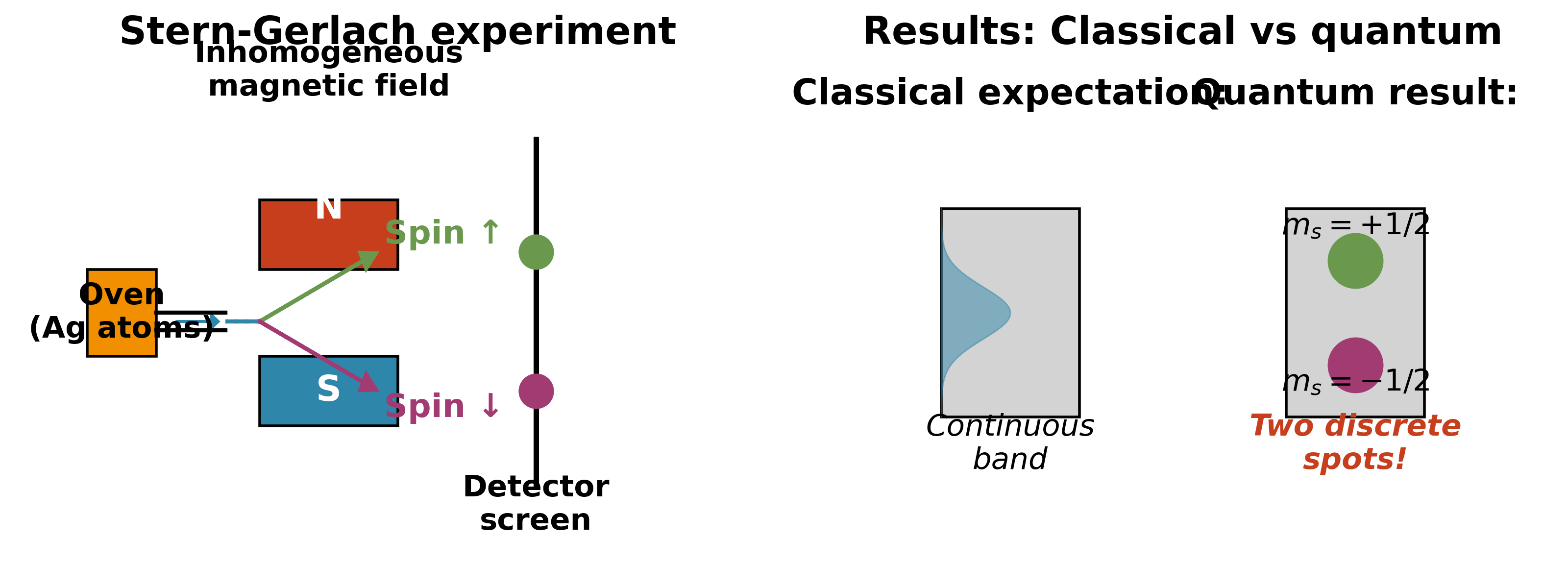
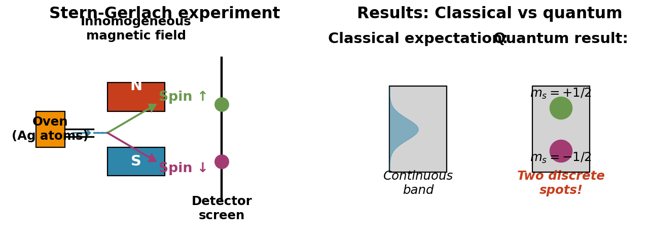
Key insight: The beam splits into exactly two components, proving that electron spin has only two possible values of \(S_z\): \(+\hbar/2\) (spin up) and \(-\hbar/2\) (spin down).

Spin-1/2: The fundamental case

Quantum numbers for spin

For spin-1/2 particles (electrons, protons, neutrons):

\[s = \frac{1}{2}, \quad m_s = -\frac{1}{2}, +\frac{1}{2}\]

The spin operators satisfy the same commutation relations as orbital angular momentum:

\[[\hat{S}_x, \hat{S}_y] = i\hbar\hat{S}_z \quad \text{(and cyclic permutations)}\]
\[\hat{S}^2 = \hat{S}_x^2 + \hat{S}_y^2 + \hat{S}_z^2\]

Eigenvalues:

\[\hat{S}^2 |\chi\rangle = \hbar^2 s(s+1) |\chi\rangle = \frac{3\hbar^2}{4} |\chi\rangle\]
\[\hat{S}_z |\chi\rangle = \hbar m_s |\chi\rangle = \pm\frac{\hbar}{2} |\chi\rangle\]
Spin states: Spinors

We denote the two spin states as:

\[\begin{split}|\uparrow\rangle = |+\rangle = \begin{pmatrix} 1 \\ 0 \end{pmatrix} \quad \text{(spin up)}\end{split}\]
\[\begin{split}|\downarrow\rangle = |-\rangle = \begin{pmatrix} 0 \\ 1 \end{pmatrix} \quad \text{(spin down)}\end{split}\]

These are called spinors – two-component vectors in spin space.

General spin state:

\[\begin{split}|\chi\rangle = \alpha|\uparrow\rangle + \beta|\downarrow\rangle = \begin{pmatrix} \alpha \\ \beta \end{pmatrix}\end{split}\]

with \(|\alpha|^2 + |\beta|^2 = 1\) (normalization).

Pauli matrices

Matrix representation of spin operators

For spin-1/2, the spin operators are represented by \(2 \times 2\) matrices:

\[\hat{S}_i = \frac{\hbar}{2}\sigma_i\]

where \(\sigma_i\) are the Pauli matrices:

\[\begin{split}\sigma_x = \begin{pmatrix} 0 & 1 \\ 1 & 0 \end{pmatrix}, \quad \sigma_y = \begin{pmatrix} 0 & -i \\ i & 0 \end{pmatrix}, \quad \sigma_z = \begin{pmatrix} 1 & 0 \\ 0 & -1 \end{pmatrix}\end{split}\]
Properties of Pauli matrices

1. Hermitian: \(\sigma_i^\dagger = \sigma_i\) (all are real, except \(\sigma_y\) has \(i\))

2. Traceless: \(\text{Tr}(\sigma_i) = 0\)

3. Unit determinant: \(\det(\sigma_i) = -1\)

4. Anticommutation: \(\{\sigma_i, \sigma_j\} = 2\delta_{ij}\) (where \(\{A,B\} = AB + BA\))

5. Commutation: \([\sigma_i, \sigma_j] = 2i\epsilon_{ijk}\sigma_k\)

6. Square to identity: \(\sigma_i^2 = I\) (the \(2\times 2\) identity matrix)

Eigenstates of Pauli matrices

For \(\sigma_z\):

\[\sigma_z |\uparrow\rangle = |\uparrow\rangle, \quad \sigma_z |\downarrow\rangle = -|\downarrow\rangle\]

For \(\sigma_x\):

\[\begin{split}|\rightarrow\rangle = \frac{1}{\sqrt{2}}(|\uparrow\rangle + |\downarrow\rangle) = \frac{1}{\sqrt{2}}\begin{pmatrix} 1 \\ 1 \end{pmatrix} \quad \text{(eigenvalue } +1\text{)}\end{split}\]
\[\begin{split}|\leftarrow\rangle = \frac{1}{\sqrt{2}}(|\uparrow\rangle - |\downarrow\rangle) = \frac{1}{\sqrt{2}}\begin{pmatrix} 1 \\ -1 \end{pmatrix} \quad \text{(eigenvalue } -1\text{)}\end{split}\]

For \(\sigma_y\):

\[\begin{split}|\circlearrowright\rangle = \frac{1}{\sqrt{2}}(|\uparrow\rangle + i|\downarrow\rangle) = \frac{1}{\sqrt{2}}\begin{pmatrix} 1 \\ i \end{pmatrix} \quad \text{(eigenvalue } +1\text{)}\end{split}\]
\[\begin{split}|\circlearrowleft\rangle = \frac{1}{\sqrt{2}}(|\uparrow\rangle - i|\downarrow\rangle) = \frac{1}{\sqrt{2}}\begin{pmatrix} 1 \\ -i \end{pmatrix} \quad \text{(eigenvalue } -1\text{)}\end{split}\]

Measuring spin in different directions

Spin is orientation-dependent

If we measure \(S_z\) on a spin-up state \(|\uparrow\rangle\):

\[\text{Result: } +\frac{\hbar}{2} \text{ with probability } 1\]

But if we measure \(S_x\) on \(|\uparrow\rangle\):

\[|\uparrow\rangle = \frac{1}{\sqrt{2}}|\rightarrow\rangle + \frac{1}{\sqrt{2}}|\leftarrow\rangle\]
\[\text{Results: } \pm\frac{\hbar}{2} \text{ each with probability } \frac{1}{2}\]

You cannot know all three components simultaneously! This is the uncertainty principle for spin.

Sequential Stern-Gerlach experiments
Experiment:
  1. Pass atoms through SG apparatus oriented in \(z\)-direction → select spin-up atoms

  2. Pass these through SG apparatus in \(x\)-direction → 50% go each way

  3. Take the \(x\)-up atoms and pass through \(z\)-direction again → 50% go each way!

Interpretation: Measuring \(S_x\) destroys information about \(S_z\). This is fundamentally different from classical physics!

General spin direction

To measure spin along an arbitrary direction \(\hat{n} = (\sin\theta\cos\phi, \sin\theta\sin\phi, \cos\theta)\):

\[\hat{S}_n = \vec{S} \cdot \hat{n} = \frac{\hbar}{2}(\sigma_x \sin\theta\cos\phi + \sigma_y \sin\theta\sin\phi + \sigma_z \cos\theta)\]

Eigenvalues are still \(\pm\hbar/2\), but eigenstates depend on \(\theta, \phi\):

\[|+_n\rangle = \cos\frac{\theta}{2}|\uparrow\rangle + e^{i\phi}\sin\frac{\theta}{2}|\downarrow\rangle\]
\[|-_n\rangle = \sin\frac{\theta}{2}|\uparrow\rangle - e^{i\phi}\cos\frac{\theta}{2}|\downarrow\rangle\]

Time evolution of spin states

Spin in a magnetic field

A spin in a magnetic field \(\vec{B} = B_0\hat{z}\) has Hamiltonian:

\[\hat{H} = -\vec{\mu} \cdot \vec{B} = -\gamma \vec{S} \cdot \vec{B} = -\gamma B_0 \hat{S}_z = -\frac{\omega_0}{2}\hbar\sigma_z\]

where \(\omega_0 = \gamma B_0\) is the Larmor frequency and \(\gamma = g e/(2m_e)\) is the gyromagnetic ratio.

Spin precession

If a spin starts in state \(|\rightarrow\rangle = (|\uparrow\rangle + |\downarrow\rangle)/\sqrt{2}\):

\[|\chi(t)\rangle = \frac{1}{\sqrt{2}}\left(e^{i\omega_0 t/2}|\uparrow\rangle + e^{-i\omega_0 t/2}|\downarrow\rangle\right)\]

The expectation values:

\[\langle S_x \rangle = \frac{\hbar}{2}\cos(\omega_0 t), \quad \langle S_y \rangle = \frac{\hbar}{2}\sin(\omega_0 t), \quad \langle S_z \rangle = 0\]

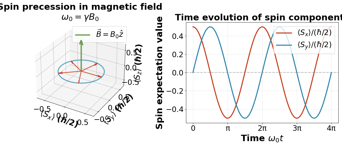
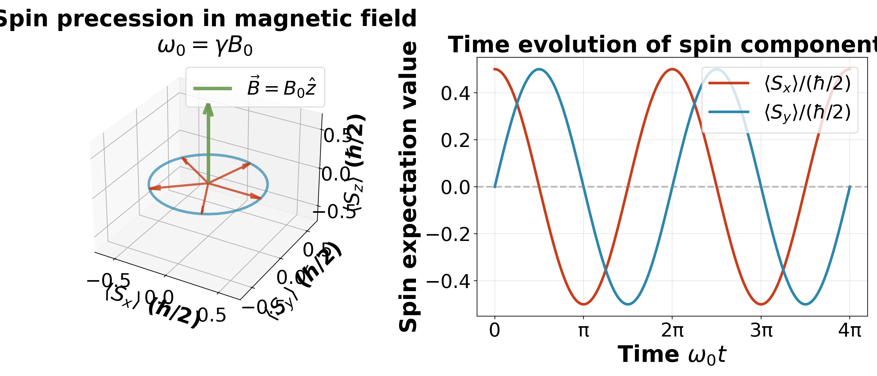
The spin precesses around the z-axis at frequency \(\omega_0\)! This is the basis for Nuclear Magnetic Resonance (NMR) and MRI.

import numpy as np
import matplotlib.pyplot as plt
from mpl_toolkits.mplot3d import Axes3D

fig = plt.figure(figsize=(14, 6))

# Left panel: Spin precession
ax1 = fig.add_subplot(121, projection='3d')

# Time points
t_vals = np.linspace(0, 2*np.pi, 50)
omega0 = 1

# Spin expectation values
Sx = 0.5 * np.cos(omega0 * t_vals)
Sy = 0.5 * np.sin(omega0 * t_vals)
Sz = np.zeros_like(t_vals)

# Plot trajectory
ax1.plot(Sx, Sy, Sz, '#2E86AB', linewidth=3, alpha=0.7)

# Plot vectors at several time points
for i in [0, 10, 20, 30, 40]:
    ax1.quiver(0, 0, 0, Sx[i], Sy[i], Sz[i], color='#C73E1D',
              arrow_length_ratio=0.2, linewidth=2.5, alpha=0.8)

# Magnetic field direction
ax1.quiver(0, 0, 0, 0, 0, 1, color='#6A994E', arrow_length_ratio=0.15,
          linewidth=4, alpha=0.9, label='$\\vec{B} = B_0\\hat{z}$')

# Formatting
ax1.set_xlabel('$\\langle S_x \\rangle$ (ℏ/2)', fontsize=24, weight='bold')
ax1.set_ylabel('$\\langle S_y \\rangle$ (ℏ/2)', fontsize=24, weight='bold')
ax1.set_zlabel('$\\langle S_z \\rangle$ (ℏ/2)', fontsize=24, weight='bold')
ax1.set_title('Spin precession in magnetic field\n$\\omega_0 = \\gamma B_0$',
             fontsize=26, weight='bold')
ax1.set_xlim([-0.7, 0.7])
ax1.set_ylim([-0.7, 0.7])
ax1.set_zlim([-0.7, 0.7])
ax1.tick_params(axis='both', labelsize=22)
ax1.legend(fontsize=22)

# Right panel: Time evolution of components
ax2 = fig.add_subplot(122)

t_plot = np.linspace(0, 4*np.pi, 200)
Sx_plot = 0.5 * np.cos(omega0 * t_plot)
Sy_plot = 0.5 * np.sin(omega0 * t_plot)

ax2.plot(t_plot, Sx_plot, '#C73E1D', linewidth=3, label='$\\langle S_x \\rangle / (\\hbar/2)$')
ax2.plot(t_plot, Sy_plot, '#2E86AB', linewidth=3, label='$\\langle S_y \\rangle / (\\hbar/2)$')
ax2.axhline(0, color='gray', linestyle='--', linewidth=2, alpha=0.5)

ax2.set_xlabel('Time $\\omega_0 t$', fontsize=26, weight='bold')
ax2.set_ylabel('Spin expectation value', fontsize=26, weight='bold')
ax2.set_title('Time evolution of spin components', fontsize=26, weight='bold')
ax2.legend(fontsize=22, loc='upper right')
ax2.grid(alpha=0.3)
ax2.tick_params(axis='both', labelsize=22)
ax2.set_xticks([0, np.pi, 2*np.pi, 3*np.pi, 4*np.pi])
ax2.set_xticklabels(['0', 'π', '2π', '3π', '4π'])

plt.tight_layout()

(Source code, png, hires.png, pdf)

../_images/quantum-1-8.png

Left: The spin expectation value \(\langle \vec{S} \rangle\) precesses around the magnetic field at the Larmor frequency.

Right: The \(x\) and \(y\) components oscillate sinusoidally, while \(\langle S_z \rangle = 0\) remains zero.

Spin and the Pauli exclusion principle

Two-particle spin states

For two spin-1/2 particles, the total spin space has dimension \(2 \times 2 = 4\). We can form:

Triplet states (\(s=1\), symmetric):

\[|1, 1\rangle = |\uparrow\uparrow\rangle\]
\[|1, 0\rangle = \frac{1}{\sqrt{2}}(|\uparrow\downarrow\rangle + |\downarrow\uparrow\rangle)\]
\[|1, -1\rangle = |\downarrow\downarrow\rangle\]

Singlet state (\(s=0\), antisymmetric):

\[|0, 0\rangle = \frac{1}{\sqrt{2}}(|\uparrow\downarrow\rangle - |\downarrow\uparrow\rangle)\]
The Pauli exclusion principle

Statement: Two identical fermions cannot occupy the same quantum state.

More precisely: The total wavefunction (space + spin) must be antisymmetric under particle exchange.

For two electrons in the same orbital (same spatial wavefunction):
  • Spatial part is symmetric

  • Spin part must be antisymmetric → singlet state \(|0,0\rangle\)

  • This is why atomic orbitals hold at most two electrons (with opposite spins)!

This explains the periodic table structure!

Spin-orbit coupling

Origin of spin-orbit interaction

In the electron’s rest frame, the nucleus appears to orbit, creating a magnetic field:

\[\vec{B} \propto \vec{L}\]

This field interacts with the electron’s magnetic moment \(\vec{\mu} \propto \vec{S}\):

\[H_{SO} = \xi(r) \vec{L} \cdot \vec{S}\]

where \(\xi(r)\) depends on the radial wavefunction.

Total angular momentum

Spin-orbit coupling means \(\vec{L}\) and \(\vec{S}\) are not separately conserved, but their sum is:

\[\vec{J} = \vec{L} + \vec{S}\]

The good quantum numbers are \((n, l, s, j, m_j)\) where:

\[j = l \pm \frac{1}{2} \quad \text{(for single electron)}\]
Fine structure in hydrogen
Spin-orbit coupling splits the \(n=2, l=1\) state (\(2p\)) into:
  • \(2p_{1/2}\): \(j = 1/2\) (2 states)

  • \(2p_{3/2}\): \(j = 3/2\) (4 states)

This creates the famous fine structure in atomic spectra, with splitting \(\Delta E \propto \alpha^2\) (where \(\alpha \approx 1/137\) is the fine structure constant).

Applications of spin

Electron spin resonance (ESR)
Flipping electron spins with microwave radiation. Used to study:
  • Free radicals in chemistry

  • Defects in semiconductors

  • Magnetic materials

Nuclear magnetic resonance (NMR) and MRI
Exploits nuclear spin (protons, :math:`^{13}`C, etc.):
  • NMR spectroscopy: Determines molecular structure

  • MRI: Medical imaging using spin precession in tissue

Spintronics
Electronics based on electron spin rather than charge:
  • GMR (giant magnetoresistance): Read heads in hard drives

  • Spin transistors

  • MRAM (magnetic RAM)

Quantum computing
Spin-1/2 systems are natural qubits:
  • Electron spins in quantum dots

  • Nuclear spins in molecules

  • NV centers in diamond

Summary: Spin

Concept

Key result

Spin quantum numbers

\(s = 1/2\); \(m_s = \pm 1/2\)

Spin operators

\(\hat{S}_i = (\hbar/2)\sigma_i\) (Pauli matrices)

Eigenvalues

\(\hat{S}^2 = (3/4)\hbar^2\); \(\hat{S}_z = \pm\hbar/2\)

Spinor states

\(|\uparrow\rangle = \binom{1}{0}\), \(|\downarrow\rangle = \binom{0}{1}\)

Pauli matrices

\(\sigma_x, \sigma_y, \sigma_z\) are \(2\times 2\) Hermitian matrices

Commutation

\([\sigma_i, \sigma_j] = 2i\epsilon_{ijk}\sigma_k\)

Precession frequency

\(\omega_0 = \gamma B_0\) (Larmor frequency)

Two-spin states

Triplet (symmetric) and singlet (antisymmetric)

Pauli exclusion

Two fermions in same orbital → singlet spin state

Spin-orbit coupling

\(H_{SO} \propto \vec{L} \cdot \vec{S}\)

We have seen how quantum mechanics describes particles using wavefunctions and the Schrödinger equation. But to truly understand quantum systems, we need a deeper mathematical framework. The concepts we develop next (eigenstates, operators, measurements) form the foundation that applies to every quantum system, whether it is an electron in an atom, a photon in a cavity, or a qubit in a quantum computer. These mathematical tools will allow us to solve any quantum problem systematically.

Mathematical foundations

Eigenstates and eigenvalues

What is an eigenstate?

In quantum mechanics, we solve eigenvalue equations of the form:

\[\hat{A} |\psi\rangle = a |\psi\rangle\]
where:
  • \(\hat{A}\): an operator (represents a physical observable like energy, momentum, position)

  • \(|\psi\rangle\): an eigenstate (a special state)

  • \(a\): an eigenvalue (a number)

Physical meaning: When the system is in eigenstate \(|\psi\rangle\), measuring observable \(\hat{A}\) always gives the value \(a\) with 100% certainty.

Example — energy eigenstates: For the Hamiltonian \(\hat{H}\):

\[\hat{H}|\psi_n\rangle = E_n |\psi_n\rangle\]

If you prepare the system in \(|\psi_n\rangle\), measuring the energy always gives \(E_n\).

Why are eigenstates important?

Two fundamental reasons:

  1. Definite measurement outcomes: Eigenstates have definite values of observables (no uncertainty)

  2. Basis for all states: ANY quantum state can be built from eigenstates (we’ll show this below)

This is why solving quantum mechanics means finding eigenstates and eigenvalues!

Different ways to represent quantum states

Before we dive deeper into operators and measurements, we need to understand a crucial point: quantum states can be represented in multiple equivalent ways. The physics is the same, but the mathematical notation differs. This often confuses students, so let’s clarify the relationships between these representations.

Dirac notation (abstract state vectors)

The notation: \(|\psi\rangle\) represents a quantum state as an abstract vector in Hilbert space.

What it means: Think of \(|\psi\rangle\) as an arrow in an infinite dimensional vector space. It doesn’t refer to any specific basis (position, momentum, energy, etc.). It is the pure, abstract quantum state itself.

Operations:
  • Inner product: \(\langle \phi | \psi \rangle\) (overlap between states, gives a complex number)

  • Outer product: \(|\psi\rangle\langle\phi|\) (gives an operator)

  • Action of operator: \(\hat{A}|\psi\rangle\) (gives another state)

Advantages:
  • Basis independent (coordinate free)

  • Makes symmetries and general principles clear

  • Compact notation for complex calculations

When to use: Abstract derivations, general theorems, operator algebra

Wavefunction notation (position representation)

The notation: \(\psi(x)\) or \(\psi(\mathbf{r})\) represents a quantum state as a function of position.

What it means: \(\psi(x)\) is the projection of the abstract state \(|\psi\rangle\) onto position eigenstates:

\[\psi(x) = \langle x | \psi \rangle\]

This answers the question: “What is the amplitude for finding the particle at position \(x\)?”

Physical interpretation: \(|\psi(x)|^2\) is the probability density for finding the particle at position \(x\).

Operations:
  • Inner product: \(\langle \phi | \psi \rangle = \int \phi^*(x) \psi(x) \, dx\)

  • Position operator: \(\hat{x}\psi(x) = x\psi(x)\) (multiplication)

  • Momentum operator: \(\hat{p}\psi(x) = -i\hbar \frac{\partial \psi}{\partial x}\) (derivative)

Advantages:
  • Concrete and visualizable

  • Direct physical interpretation (\(|\psi(x)|^2\) is measurable)

  • Natural for solving differential equations (Schrödinger equation)

When to use: Solving specific problems, visualizing wavefunctions, connecting to experiments

Matrix representation (discrete basis)

The notation:

\[\begin{split}|\psi\rangle = \begin{pmatrix} c_1 \\ c_2 \\ c_3 \\ \vdots \end{pmatrix}, \quad \hat{A} = \begin{pmatrix} A_{11} & A_{12} & \cdots \\ A_{21} & A_{22} & \cdots \\ \vdots & \vdots & \ddots \end{pmatrix}\end{split}\]

What it means: Represent states as column vectors and operators as matrices in some chosen basis (usually energy eigenstates).

Connection to Dirac notation: If we expand in basis states \(\{|\phi_n\rangle\}\):

\[\begin{split}|\psi\rangle = \sum_n c_n |\phi_n\rangle \quad \Leftrightarrow \quad |\psi\rangle = \begin{pmatrix} c_1 \\ c_2 \\ c_3 \\ \vdots \end{pmatrix}\end{split}\]

where \(c_n = \langle \phi_n | \psi \rangle\) are the expansion coefficients.

Operations:
  • Inner product: \(\langle \phi | \psi \rangle = \phi^\dagger \psi\) (matrix multiplication)

  • Operator action: \(\hat{A}|\psi\rangle = A\psi\) (matrix times vector)

  • Expectation value: \(\langle \psi | \hat{A} | \psi \rangle = \psi^\dagger A \psi\)

Advantages:
  • Finite dimensional → numerical computation

  • Linear algebra techniques apply directly

  • Natural for quantum computing (qubits are 2D vectors)

  • Clear connection to eigenvalue problems

When to use: Numerical calculations, finite systems, quantum computing, computational physics

Momentum representation

The notation: \(\tilde{\psi}(p)\) or \(\phi(p)\) represents a quantum state as a function of momentum.

What it means: \(\tilde{\psi}(p) = \langle p | \psi \rangle\) is the amplitude for finding the particle with momentum \(p\).

Connection to position representation: They are related by Fourier transform:

\[\tilde{\psi}(p) = \frac{1}{\sqrt{2\pi\hbar}} \int_{-\infty}^{\infty} e^{-ipx/\hbar} \psi(x) \, dx\]
\[\psi(x) = \frac{1}{\sqrt{2\pi\hbar}} \int_{-\infty}^{\infty} e^{ipx/\hbar} \tilde{\psi}(p) \, dp\]

Physical interpretation: \(|\tilde{\psi}(p)|^2\) is the probability density for measuring momentum \(p\).

Operations:
  • Position operator: \(\hat{x}\tilde{\psi}(p) = i\hbar \frac{\partial \tilde{\psi}}{\partial p}\) (derivative in momentum space!)

  • Momentum operator: \(\hat{p}\tilde{\psi}(p) = p\tilde{\psi}(p)\) (multiplication in momentum space)

When to use: Problems with simple momentum structure, scattering theory, free particles

How they all connect: The same state in different languages

Let’s see how the same quantum state appears in different representations using a concrete example.

Example: Consider the first excited state of a particle in a box of length \(L\).

Dirac notation (abstract):

\[|\psi\rangle = |2\rangle\]

This just names the state without specifying any coordinates.

Wavefunction (position representation):

\[\psi(x) = \langle x | 2 \rangle = \sqrt{\frac{2}{L}} \sin\left(\frac{2\pi x}{L}\right)\]

This tells us the amplitude at each position \(x\).

Matrix representation (energy basis):

\[\begin{split}|\psi\rangle = \begin{pmatrix} 0 \\ 1 \\ 0 \\ 0 \\ \vdots \end{pmatrix}\end{split}\]

This shows \(c_1 = 0\), \(c_2 = 1\), \(c_3 = 0\), etc. (only the second energy level is occupied).

Momentum representation (Fourier transform):

\[\tilde{\psi}(p) = \langle p | 2 \rangle = \text{(complicated expression involving momentum)}\]

They are all the same state! Just expressed in different “coordinate systems.”

Converting between representations

Key formula: The wavefunction is the inner product with position eigenstates:

\[\psi(x) = \langle x | \psi \rangle\]

Expanding in a basis: If \(\{|\phi_n\rangle\}\) form a complete basis:

\[|\psi\rangle = \sum_n c_n |\phi_n\rangle \quad \text{where} \quad c_n = \langle \phi_n | \psi \rangle\]

In position space:

\[\psi(x) = \sum_n c_n \phi_n(x) \quad \text{where} \quad \phi_n(x) = \langle x | \phi_n \rangle\]

The completeness relation:

\[\int |x\rangle\langle x| \, dx = \hat{I} \quad \text{(identity operator)}\]

This expresses the fact that integrating over all positions gives you back the complete state.

Why does this matter?

Different problems are easier in different representations:

  • Free particle: Momentum representation (plane waves \(e^{ipx/\hbar}\))

  • Harmonic oscillator: Energy basis (ladder operators)

  • Particle in a box: Position representation (boundary conditions)

  • Quantum computing: Matrix representation (2×2 matrices for qubits)

The physics doesn’t change:
  • \(\langle \psi | \hat{A} | \psi \rangle\) is the same number regardless of representation

  • Eigenvalues are the same (these are measurable quantities!)

  • Transition probabilities \(|\langle \phi | \psi \rangle|^2\) are the same

You can switch representations anytime: If you get stuck in one representation, try another! Fourier transforming between position and momentum is often useful.

Example: Expectation value in all three forms

The same calculation in different notations:

Calculate \(\langle x \rangle\) (average position) for a state \(|\psi\rangle\).

Dirac notation (abstract):

\[\langle x \rangle = \langle \psi | \hat{x} | \psi \rangle\]

Wavefunction (position representation):

\[\langle x \rangle = \int_{-\infty}^{\infty} \psi^*(x) \, x \, \psi(x) \, dx\]

Matrix representation (discrete basis \(\{|\phi_n\rangle\}\)):

\[\langle x \rangle = \sum_{m,n} c_m^* X_{mn} c_n \quad \text{where} \quad X_{mn} = \langle \phi_m | \hat{x} | \phi_n \rangle\]

Or in matrix form:

\[\langle x \rangle = \psi^\dagger X \psi\]

All three give the same number! The first is most compact, the second most intuitive, the third most computational.

Quick reference: Representation cheat sheet

Representation

State notation

Inner product

Operator action

Dirac (abstract)

\(|\psi\rangle\)

\(\langle \phi | \psi \rangle\)

\(\hat{A}|\psi\rangle\)

Wavefunction

\(\psi(x)\)

\(\int \phi^*(x)\psi(x)dx\)

\(\hat{A}\psi(x)\)

Matrix

\(\begin{pmatrix}c_1\\c_2\\\vdots\end{pmatrix}\)

\(\phi^\dagger\psi\)

\(A\psi\)

Momentum

\(\tilde{\psi}(p)\)

\(\int \tilde{\phi}^*(p)\tilde{\psi}(p)dp\)

\(\hat{A}\tilde{\psi}(p)\)

Bottom line: These are all equivalent ways to describe quantum mechanics. Master them all, and you can tackle any problem in the representation that makes it simplest!

Hermitian operators

What operators represent physical observables?

In quantum mechanics, physical observables (energy, momentum, position) are represented by Hermitian operators. An operator \(\hat{A}\) is Hermitian if:

\[\langle \psi | \hat{A} \phi \rangle = \langle \hat{A} \psi | \phi \rangle\]

for all wavefunctions \(\psi\) and \(\phi\).

In integral form:

\[\int \psi^* \hat{A} \phi \, d^3r = \int (\hat{A} \psi)^* \phi \, d^3r\]

Convention: Operators are applied to the state on their right. In \(\langle \psi | \hat{A} \phi \rangle\), the operator \(\hat{A}\) acts on \(|\phi\rangle\) (to the right), giving \(\hat{A}|\phi\rangle\), and then we take the inner product with \(\langle \psi |\).

Why must observables be Hermitian?

Because measurements must yield real values! Hermitian operators guarantee:

  1. All eigenvalues are real (proven below)

  2. Eigenstates with different eigenvalues are orthogonal (proven below)

These properties are essential for quantum mechanics to make sense physically.

Proving \(\langle \phi | A \psi \rangle = \langle A \phi | \psi \rangle\)

This property is the key to proving that Hermitian operators have real eigenvalues. Let’s see why this equation holds using matrix form, which is how we actually work with quantum systems in practice (finite basis sets, computational calculations, etc.).

The matrix definition of Hermitian

A Hermitian matrix \(A\) satisfies:

\[A = A^\dagger = (A^T)^*\]

This means taking the transpose and complex conjugate gives you back the same matrix.

Starting with the inner product

For two column vectors \(\phi\) and \(\psi\), their inner product is:

\[\langle \phi | \psi \rangle = \phi^\dagger \psi\]

When you apply operator \(A\) to the right vector:

\[\langle \phi | A \psi \rangle = \phi^\dagger A \psi\]

The algebraic manipulation

Take the complex conjugate of this entire expression:

\[(\langle \phi | A \psi \rangle)^* = (\phi^\dagger A \psi)^* = \psi^\dagger A^\dagger \phi\]

Here’s where the Hermitian property becomes useful. Since \(A^\dagger = A\):

\[(\langle \phi | A \psi \rangle)^* = \psi^\dagger A \phi = \langle \psi | A \phi \rangle\]

Taking the complex conjugate one more time:

\[\langle \phi | A \psi \rangle = \langle A \phi | \psi \rangle\]

What this means: You can “move” the operator \(A\) across the inner product from the right side to the left side. This algebraic property is exactly what we’ll use below to prove that eigenvalues must be real.

Properties of Hermitian operators

Property 1: Real eigenvalues

Theorem: If \(\hat{H}\) is a Hermitian operator, then all its eigenvalues are real.

Setup: Suppose \(|\psi\rangle\) is an eigenstate with eigenvalue \(\lambda\):

\[\hat{H}|\psi\rangle = \lambda |\psi\rangle\]

What we’ll prove: \(\lambda = \lambda^*\) (real number)

Proof strategy: Compute \(\langle \psi | \hat{H} | \psi \rangle\) two different ways and compare.

First way — using the eigenvalue equation directly:

\[\langle \psi | \hat{H} | \psi \rangle = \langle \psi | \lambda \psi \rangle = \lambda \langle \psi | \psi \rangle\]

Second way — using the Hermitian property \(\langle \psi | \hat{H} \psi \rangle = \langle \hat{H} \psi | \psi \rangle\):

\[\langle \psi | \hat{H} | \psi \rangle = \langle \hat{H} \psi | \psi \rangle = \langle \lambda \psi | \psi \rangle = \lambda^* \langle \psi | \psi \rangle\]

(The scalar becomes conjugated when moved to the bra)

Equating both expressions:

\[\lambda \langle \psi | \psi \rangle = \lambda^* \langle \psi | \psi \rangle\]

Since \(\langle \psi | \psi \rangle \neq 0\):

\[\boxed{\lambda = \lambda^*}\]

Therefore \(\lambda\) is real!

Physical meaning: Measurements always give real numbers, never imaginary ones. This is why observables must be Hermitian.

Property 2: Orthogonal eigenstates

Theorem: Eigenstates with different eigenvalues are orthogonal.

Setup: Two eigenstates with different eigenvalues:

\[\hat{H}|\psi_1\rangle = \lambda_1 |\psi_1\rangle, \quad \hat{H}|\psi_2\rangle = \lambda_2 |\psi_2\rangle, \quad \lambda_1 \neq \lambda_2\]

Proof: Compute \(\langle \psi_1 | \hat{H} | \psi_2 \rangle\) two ways:

Using the right eigenvalue:

\[\langle \psi_1 | \hat{H} | \psi_2 \rangle = \lambda_2 \langle \psi_1 | \psi_2 \rangle\]

Using the Hermitian property and left eigenvalue:

\[\langle \psi_1 | \hat{H} | \psi_2 \rangle = \langle \hat{H} \psi_1 | \psi_2 \rangle = \lambda_1 \langle \psi_1 | \psi_2 \rangle\]

(Using \(\lambda_1^* = \lambda_1\) since eigenvalues are real)

Equating:

\[\lambda_2 \langle \psi_1 | \psi_2 \rangle = \lambda_1 \langle \psi_1 | \psi_2 \rangle\]
\[(\lambda_2 - \lambda_1) \langle \psi_1 | \psi_2 \rangle = 0\]

Since \(\lambda_1 \neq \lambda_2\):

\[\boxed{\langle \psi_1 | \psi_2 \rangle = 0}\]

Physical meaning: Different energy states don’t “mix” — they’re completely separate. This is fundamental to quantum mechanics.

Note: If \(\lambda_1 = \lambda_2\) (degenerate eigenvalues), eigenstates aren’t automatically orthogonal, but can be made orthogonal using Gram-Schmidt.

Expansion in eigenstates

The completeness relation

Key result: The eigenstates of a Hermitian operator form an orthonormal basis. ANY quantum state can be written as:

\[|\psi\rangle = \sum_n c_n |\phi_n\rangle\]

where \(|\phi_n\rangle\) are eigenstates and \(c_n\) are coefficients.

Finding the coefficients

Use orthonormality \(\langle \phi_m | \phi_n \rangle = \delta_{mn}\):

\[c_n = \langle \phi_n | \psi \rangle = \int \phi_n^*(x) \psi(x) \, dx\]

This is the projection — it extracts how much of eigenstate \(|\phi_n\rangle\) is in \(|\psi\rangle\).

Let’s work through a 3D example to see projection in action with multiple states.

Setup: Suppose we have three orthonormal basis states:

\[\begin{split}|\phi_1\rangle = \begin{pmatrix} 1 \\ 0 \\ 0 \end{pmatrix}, \quad |\phi_2\rangle = \begin{pmatrix} 0 \\ 1 \\ 0 \end{pmatrix}, \quad |\phi_3\rangle = \begin{pmatrix} 0 \\ 0 \\ 1 \end{pmatrix}\end{split}\]

And a quantum state:

\[\begin{split}|\psi\rangle = \begin{pmatrix} 0.5 \\ 0.7 \\ 0.5 \end{pmatrix}\end{split}\]

Check normalization: \(|0.5|^2 + |0.7|^2 + |0.5|^2 = 0.25 + 0.49 + 0.25 = 0.99 \approx 1\)

(Using 0.99 to keep numbers simple; in practice we’d normalize exactly)

Finding the coefficients using projection:

\[\begin{split}c_1 = \langle \phi_1 | \psi \rangle = \begin{pmatrix} 1 & 0 & 0 \end{pmatrix} \begin{pmatrix} 0.5 \\ 0.7 \\ 0.5 \end{pmatrix} = 0.5\end{split}\]
\[\begin{split}c_2 = \langle \phi_2 | \psi \rangle = \begin{pmatrix} 0 & 1 & 0 \end{pmatrix} \begin{pmatrix} 0.5 \\ 0.7 \\ 0.5 \end{pmatrix} = 0.7\end{split}\]
\[\begin{split}c_3 = \langle \phi_3 | \psi \rangle = \begin{pmatrix} 0 & 0 & 1 \end{pmatrix} \begin{pmatrix} 0.5 \\ 0.7 \\ 0.5 \end{pmatrix} = 0.5\end{split}\]

Reconstruction: We can write:

\[|\psi\rangle = 0.5 |\phi_1\rangle + 0.7 |\phi_2\rangle + 0.5 |\phi_3\rangle\]
\[\begin{split}= 0.5 \begin{pmatrix} 1 \\ 0 \\ 0 \end{pmatrix} + 0.7 \begin{pmatrix} 0 \\ 1 \\ 0 \end{pmatrix} + 0.5 \begin{pmatrix} 0 \\ 0 \\ 1 \end{pmatrix} = \begin{pmatrix} 0.5 \\ 0.7 \\ 0.5 \end{pmatrix} \quad ✓\end{split}\]

Measurement probabilities:

  • Probability of measuring \(\lambda_1\): \(|c_1|^2 = 0.25 = 25\%\)

  • Probability of measuring \(\lambda_2\): \(|c_2|^2 = 0.49 = 49\%\)

  • Probability of measuring \(\lambda_3\): \(|c_3|^2 = 0.25 = 25\%\)

  • Total: \(0.25 + 0.49 + 0.25 = 0.99 \approx 100\%\)

Physical interpretation: State \(|\psi\rangle\) is a superposition where the system has:

  • 25% chance of being in state \(|\phi_1\rangle\)

  • 49% chance of being in state \(|\phi_2\rangle\) (most likely!)

  • 25% chance of being in state \(|\phi_3\rangle\)

The projection \(c_n = \langle \phi_n | \psi \rangle\) extracts each component’s amplitude.

(Source code, png, hires.png, pdf)

../_images/quantum-1-9.png

Physical interpretation

  • \(|c_n|^2\) = probability of measuring eigenvalue \(\lambda_n\)

  • Before measurement: superposition of all eigenstates

  • After measurement: collapses to one eigenstate

  • Normalization: \(\sum_n |c_n|^2 = 1\)

Time evolution

For energy eigenstates \(\hat{H}|\psi_n\rangle = E_n|\psi_n\rangle\):

\[|\psi(t)\rangle = \sum_n c_n e^{-iE_n t/\hbar} |\psi_n\rangle\]

Each eigenstate picks up its own time-dependent phase!

Matrix representation

In a finite basis (quantum computing, numerical calculations):

\[\begin{split}|\psi\rangle = \begin{pmatrix} c_1 \\ c_2 \\ \vdots \\ c_n \end{pmatrix}, \quad |\phi_1\rangle = \begin{pmatrix} 1 \\ 0 \\ \vdots \\ 0 \end{pmatrix}, \quad |\phi_2\rangle = \begin{pmatrix} 0 \\ 1 \\ \vdots \\ 0 \end{pmatrix}\end{split}\]

This is how we actually compute in practice!

Measurements and expectation values

The measurement postulate

When you measure an observable \(\hat{A}\) on a system in state \(|\psi\rangle\), here’s what happens:

Step 1: Your state is a superposition

First, remember that ANY state \(|\psi\rangle\) can be written as a superposition of the eigenstates \(|\phi_n\rangle\) of the operator \(\hat{A}\):

\[|\psi\rangle = c_1 |\phi_1\rangle + c_2 |\phi_2\rangle + c_3 |\phi_3\rangle + \cdots = \sum_n c_n |\phi_n\rangle\]

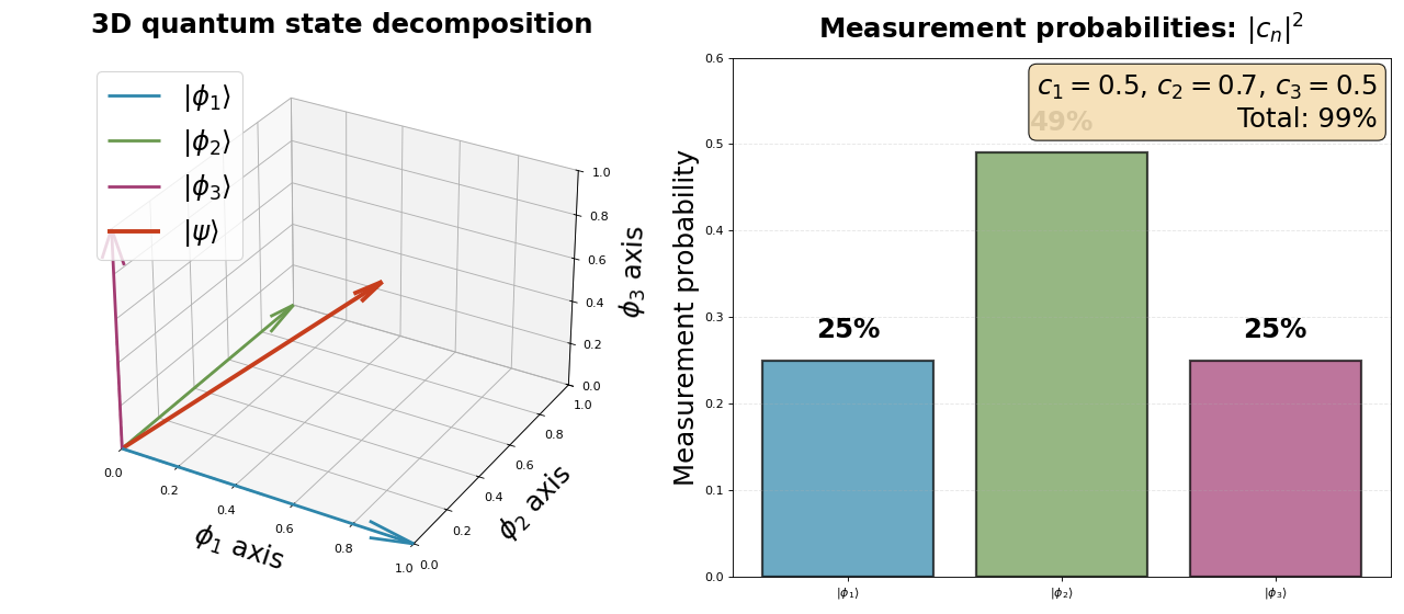
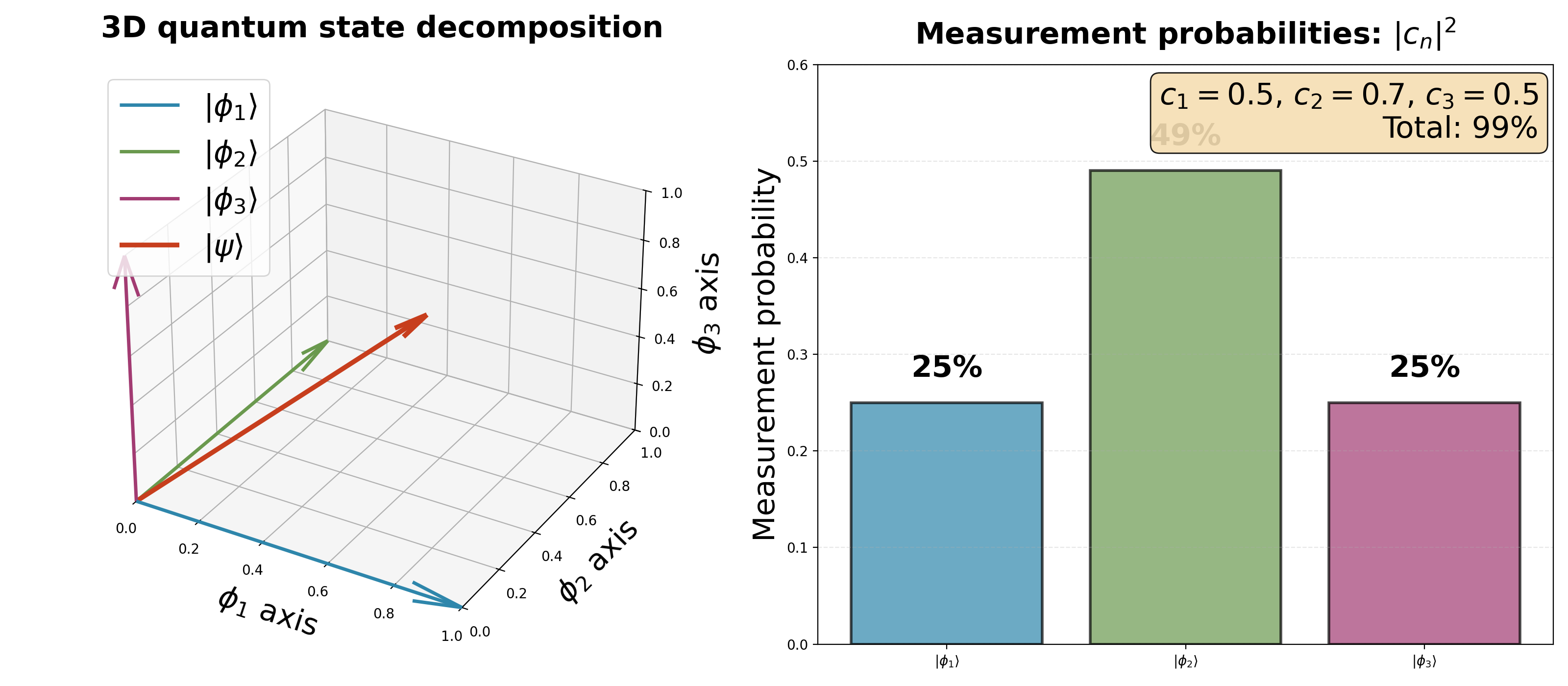
Think of it like this: the eigenstates \(|\phi_n\rangle\) are like basis vectors (north, east, up), and your state \(|\psi\rangle\) is built from these pieces. The coefficients \(c_n\) tell you “how much” of each eigenstate is in your state.

Step 2: Finding the coefficients (projection)

How do we find \(c_n\)? We use the inner product (projection):

\[c_n = \langle \phi_n | \psi \rangle = \int \phi_n^* \psi \, d^3r\]

This is literally the overlap between \(|\phi_n\rangle\) and \(|\psi\rangle\). If your state \(|\psi\rangle\) looks a lot like \(|\phi_n\rangle\), then \(c_n\) is large. If they’re perpendicular (orthogonal), then \(c_n = 0\).

Example: If \(|\psi\rangle = 0.6|\phi_1\rangle + 0.8|\phi_2\rangle\), then:

  • \(c_1 = \langle \phi_1 | \psi \rangle = 0.6\)

  • \(c_2 = \langle \phi_2 | \psi \rangle = 0.8\)

The projection “extracts” each component from the superposition!

Step 3: Measurement outcomes and probabilities

When you measure \(\hat{A}\):

  • You will get one of the eigenvalues \(a_n\) (NOT a superposition of values!)

  • The probability of getting \(a_n\) is \(|c_n|^2\)

  • After the measurement, the system “collapses” to \(|\phi_n\rangle\)

Continuing the example: For \(|\psi\rangle = 0.6|\phi_1\rangle + 0.8|\phi_2\rangle\):

  • Probability of measuring \(a_1\): \(|c_1|^2 = |0.6|^2 = 0.36 = 36\%\)

  • Probability of measuring \(a_2\): \(|c_2|^2 = |0.8|^2 = 0.64 = 64\%\)

  • Total probability: \(0.36 + 0.64 = 1\)

The key insight: Before measurement, the system is in a superposition (both states at once). After measurement, it’s definitely in one eigenstate. The coefficients \(c_n\) from the superposition determine the measurement probabilities!

This is why we needed real eigenvalues (Hermitian operators) and orthogonal eigenstates!

Expectation values — the average of many measurements

If you repeat the same measurement many times on identically prepared systems, the average result is:

\[\langle \hat{A} \rangle = \langle \psi | \hat{A} | \psi \rangle = \int \psi^* \hat{A} \psi \, d^3r\]

In matrix form (using a finite basis):

\[\langle \hat{A} \rangle = \psi^\dagger A \psi = \sum_{i,j} \psi_i^* A_{ij} \psi_j\]

This is the expectation value of operator \(\hat{A}\) in state \(|\psi\rangle\).

Example — position and momentum expectation values:

\[\langle x \rangle = \int \psi^* x \psi \, dx \quad \text{(average position)}\]
\[\langle p \rangle = \int \psi^* \left(-i\hbar \frac{\partial}{\partial x}\right) \psi \, dx \quad \text{(average momentum)}\]

Connection to eigenstates: If \(|\psi\rangle\) is an eigenstate of \(\hat{A}\) with eigenvalue \(a\), then every measurement gives \(a\) with certainty:

\[\langle \hat{A} \rangle = \langle \psi | \hat{A} | \psi \rangle = \langle \psi | a \psi \rangle = a \langle \psi | \psi \rangle = a\]

This is why finding eigenstates and eigenvalues is so important — they represent states with definite values of observables.

Commutators and compatible observables

What is a commutator?

The commutator of two operators \(\hat{A}\) and \(\hat{B}\) measures whether they can be measured simultaneously:

\[[\hat{A}, \hat{B}] = \hat{A}\hat{B} - \hat{B}\hat{A}\]

If \([\hat{A}, \hat{B}] = 0\), we say the operators commute. If \([\hat{A}, \hat{B}] \neq 0\), they don’t commute.

Physical meaning:

  • If \([\hat{A}, \hat{B}] = 0\): The observables can be measured simultaneously with perfect precision. They share eigenstates.

  • If \([\hat{A}, \hat{B}] \neq 0\): Cannot simultaneously know both with certainty. This is the origin of uncertainty relations.

The most famous commutator — position and momentum:

\[[\hat{x}, \hat{p}] = i\hbar\]

Let’s derive this. Using \(\hat{p} = -i\hbar \frac{\partial}{\partial x}\), apply both operators to a test function \(\psi\):

\[\hat{x}\hat{p}\psi = \hat{x}\left(-i\hbar \frac{\partial \psi}{\partial x}\right) = -i\hbar x \frac{\partial \psi}{\partial x}\]
\[\hat{p}\hat{x}\psi = -i\hbar \frac{\partial}{\partial x}(x\psi) = -i\hbar \left(\psi + x\frac{\partial \psi}{\partial x}\right)\]

Subtract:

\[[\hat{x}, \hat{p}]\psi = -i\hbar x \frac{\partial \psi}{\partial x} - \left(-i\hbar \psi - i\hbar x\frac{\partial \psi}{\partial x}\right) = i\hbar \psi\]

Therefore:

\[\boxed{[\hat{x}, \hat{p}] = i\hbar}\]

What this means: You cannot simultaneously know position and momentum with perfect precision. This is Heisenberg’s uncertainty principle.

The uncertainty principle

Heisenberg’s uncertainty principle is not just a statement about measurement limitations — it’s a fundamental property of quantum mechanics arising from commutators.

The general uncertainty relation

For any two observables \(\hat{A}\) and \(\hat{B}\), the uncertainties \(\Delta A\) and \(\Delta B\) satisfy:

\[\Delta A \cdot \Delta B \geq \frac{1}{2} |\langle [\hat{A}, \hat{B}] \rangle|\]

where the uncertainty is defined as the standard deviation:

\[\Delta A = \sqrt{\langle \hat{A}^2 \rangle - \langle \hat{A} \rangle^2}\]
Proof of the general uncertainty relation

This is a beautiful result that follows from the Cauchy-Schwarz inequality. Let’s derive it step by step.

Step 1: Define shifted operators

Define operators shifted by their expectation values:

\[\Delta\hat{A} = \hat{A} - \langle \hat{A} \rangle, \quad \Delta\hat{B} = \hat{B} - \langle \hat{B} \rangle\]

These represent deviations from the mean. The uncertainties are:

\[(\Delta A)^2 = \langle (\Delta\hat{A})^2 \rangle, \quad (\Delta B)^2 = \langle (\Delta\hat{B})^2 \rangle\]

Step 2: Apply Cauchy-Schwarz inequality

For any two operators \(\hat{X}\) and \(\hat{Y}\):

\[|\langle \psi | \hat{X}^\dagger \hat{Y} | \psi \rangle|^2 \leq \langle \psi | \hat{X}^\dagger \hat{X} | \psi \rangle \langle \psi | \hat{Y}^\dagger \hat{Y} | \psi \rangle\]

Apply this with \(\hat{X} = \Delta\hat{A}\) and \(\hat{Y} = \Delta\hat{B}\) (noting these are Hermitian):

\[|\langle \Delta\hat{A} \Delta\hat{B} \rangle|^2 \leq \langle (\Delta\hat{A})^2 \rangle \langle (\Delta\hat{B})^2 \rangle = (\Delta A)^2 (\Delta B)^2\]

Step 3: Decompose into commutator and anticommutator

Any product can be written as:

\[\Delta\hat{A} \Delta\hat{B} = \frac{1}{2}\{\Delta\hat{A}, \Delta\hat{B}\} + \frac{1}{2}[\Delta\hat{A}, \Delta\hat{B}]\]

where \(\{\hat{A}, \hat{B}\} = \hat{A}\hat{B} + \hat{B}\hat{A}\) is the anticommutator.

Taking expectation values:

\[\langle \Delta\hat{A} \Delta\hat{B} \rangle = \frac{1}{2}\langle \{\Delta\hat{A}, \Delta\hat{B}\} \rangle + \frac{1}{2}\langle [\Delta\hat{A}, \Delta\hat{B}] \rangle\]

The anticommutator part is real, the commutator part is purely imaginary (for Hermitian operators).

Step 4: Use triangle inequality

The magnitude satisfies:

\[|\langle \Delta\hat{A} \Delta\hat{B} \rangle| \geq \frac{1}{2}|\langle [\Delta\hat{A}, \Delta\hat{B}] \rangle|\]

Step 5: Note that the commutators are equal

\[[\Delta\hat{A}, \Delta\hat{B}] = [\hat{A} - \langle \hat{A} \rangle, \hat{B} - \langle \hat{B} \rangle] = [\hat{A}, \hat{B}]\]

(Constants commute with everything, so they drop out)

Step 6: Combine everything

From steps 2 and 4:

\[(\Delta A)^2 (\Delta B)^2 \geq |\langle \Delta\hat{A} \Delta\hat{B} \rangle|^2 \geq \frac{1}{4}|\langle [\hat{A}, \hat{B}] \rangle|^2\]

Taking the square root:

\[\boxed{\Delta A \cdot \Delta B \geq \frac{1}{2} |\langle [\hat{A}, \hat{B}] \rangle|}\]

Physical interpretation: The uncertainty product is bounded by the commutator. Non-commuting observables cannot both be precisely known!

Position-momentum uncertainty

Using \([\hat{x}, \hat{p}] = i\hbar\):

\[\boxed{\Delta x \cdot \Delta p \geq \frac{\hbar}{2}}\]

This is the famous Heisenberg uncertainty principle.

Physical interpretation:

  • You cannot prepare a state where both position and momentum are precisely defined

  • The more localized the wavefunction (small \(\Delta x\)), the more spread out in momentum space (large \(\Delta p\))

  • This is not about measurement disturbing the system — it’s about the wave nature of matter

  • A plane wave \(e^{ikx}\) has definite momentum (\(\Delta p = 0\)) but completely undefined position (\(\Delta x = \infty\))

  • A localized wavepacket has finite \(\Delta x\), so it must have finite \(\Delta p\)

Example — particle in a box:

For the ground state of a particle in a box of width \(L\), we can estimate:

  • \(\Delta x \sim L\) (particle is somewhere in the box)

  • From uncertainty: \(\Delta p \gtrsim \hbar/L\)

  • Kinetic energy: \(E \sim \frac{p^2}{2m} \sim \frac{(\hbar/L)^2}{2m} = \frac{\hbar^2}{2mL^2}\)

This matches the exact ground state energy \(E_1 = \frac{\hbar^2 \pi^2}{2mL^2}\) within a factor of \(\pi^2 \approx 10\)!

Summary: Why these mathematical foundations matter

Everything we’ve covered forms the complete mathematical framework for quantum mechanics:

1. Eigenstates and eigenvalues: The foundation
  • States with definite measurement outcomes

  • Solving QM = finding eigenstates

2. Hermitian operators: What represents observables
  • Ensure real eigenvalues (physical measurements)

  • Ensure orthogonal eigenstates (no mixing)

3. Expansion in eigenstates: Building any state
  • Any state = superposition of eigenstates

  • Coefficients determine measurement probabilities

4. Measurements: Connecting math to experiments
  • Measurement outcomes = eigenvalues

  • Probabilities from superposition coefficients

  • Expectation values for repeated measurements

5. Commutators and uncertainty: Fundamental limits
  • Non-commuting operators can’t be simultaneously known

  • Uncertainty relations from wave-particle duality

Every quantum system (particle in a box, harmonic oscillator, hydrogen atom, quantum computer) uses these principles!

Now that we understand the mathematical foundations (eigenstates, Hermitian operators, measurements, and uncertainty relations), let’s see these principles in action with real quantum systems. We will start with the simplest example: a particle confined to a one dimensional box. This seemingly simple problem contains all the essential features of quantum mechanics: wave particle duality, quantized energy levels, and probability interpretation. Once we master this, we can tackle more complex systems using the same mathematical machinery.

Particle in a box

Why start with this problem?

Why is the particle in a box the first quantum mechanics problem we solve?

The particle in a box is the simplest non-trivial quantum system that demonstrates energy quantization. Here’s why it’s pedagogically important:

1. Simplest potential with bound states

The potential is trivial inside the box (\(V = 0\)), so we only deal with the kinetic energy term of the Schrödinger equation:

\[-\frac{\hbar^2}{2m} \frac{d^2\psi}{dx^2} = E \psi\]

There’s no complicated potential function to worry about. This is the minimum complexity needed to see quantization.

2. First system with boundary conditions

The infinite walls at \(x = 0\) and \(x = L\) impose boundary conditions: \(\psi(0) = \psi(L) = 0\).

These boundary conditions force quantization. Not all wavelengths fit in the box—only those satisfying the boundary conditions are allowed. This is the physical origin of discrete energy levels.

3. Builds intuition for all quantum systems
Concepts learned here apply everywhere:
  • Standing waves → energy eigenstates

  • Boundary conditions → quantization

  • Wave nature → probability interpretation

  • Nodes and antinodes → wavefunction structure

4. Analytically solvable

The solution involves only trigonometric functions (\(\sin\), \(\cos\)). No special functions (Bessel, Hermite, etc.) are needed. This lets us focus on physical concepts rather than mathematical machinery.

5. Real physical applications
Despite its simplicity, this model describes:
  • Electrons in quantum dots (nanoscale semiconductor crystals)

  • Conjugated π-electrons in molecules (particle-in-a-box approximation)

  • Nucleons in nuclear shell model

  • Conduction electrons in 1D nanowires

Why not start with the hydrogen atom?
The hydrogen atom is physically more important (it’s a real atom!), but mathematically much harder:
  • Requires spherical coordinates

  • Needs special functions (Laguerre polynomials, spherical harmonics)

  • Three quantum numbers instead of one

  • Coulomb potential \(V(r) = -e^2/(4\pi\epsilon_0 r)\) is more complex

The particle in a box teaches the same fundamental concepts (quantization, wavefunctions, probability) with simpler mathematics.

The infinite square well

What is the particle in a box problem?

A particle is confined to a one-dimensional box of length \(L\). The potential is:

\[\begin{split}V(x) = \begin{cases} 0 & \text{if } 0 < x < L \\ \infty & \text{otherwise} \end{cases}\end{split}\]

Physical meaning: The particle cannot escape the box (infinite walls). Inside the box, it moves freely.

(Source code, png, hires.png, pdf)

../_images/plot_particle_in_box_potential.png

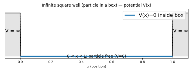
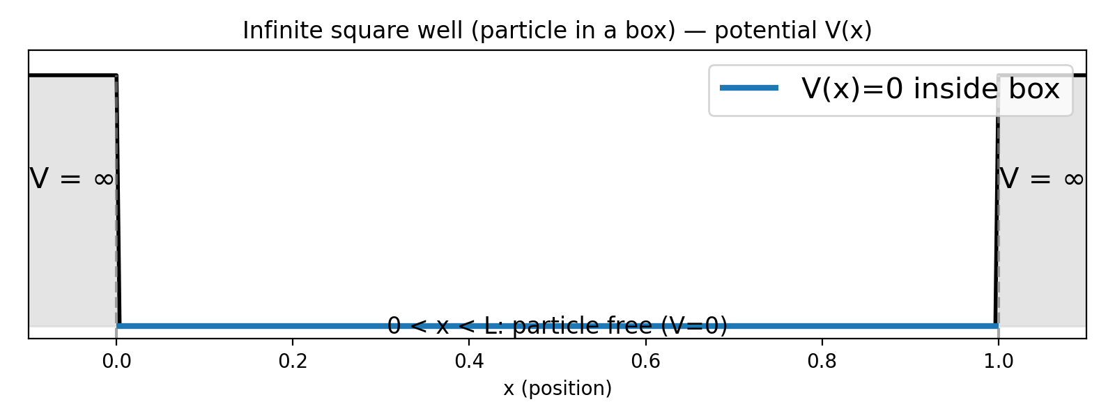
The figure above shows the infinite square well potential used in the particle-in-a-box model: \(V(x)=0\) for \(0 < x < L\) and \(V(x)=\infty\) outside. This is the model/postulate that enforces the boundary conditions \(\psi(0)=\psi(L)=0\) (the particle cannot be found where the potential is infinite).

What are the boundary conditions?

Since \(V = \infty\) outside the box, the wavefunction must vanish at the walls:

\[\psi(0) = 0 \quad \text{and} \quad \psi(L) = 0\]

Why? The probability of finding the particle outside must be zero. The wavefunction must be continuous, so \(\psi = 0\) at the boundaries.

What are the allowed energy levels?

Inside the box, the time-independent Schrödinger equation is:

\[-\frac{\hbar^2}{2m} \frac{d^2\psi}{dx^2} = E \psi\]

Step 1: Rewrite the equation

Rearrange:

\[\frac{d^2\psi}{dx^2} = -\frac{2mE}{\hbar^2} \psi\]

Define \(k^2 = \frac{2mE}{\hbar^2}\), so:

\[\frac{d^2\psi}{dx^2} = -k^2 \psi\]

This is a standard second-order differential equation with constant coefficients.

Step 2: General solution

The general solution is:

\[\psi(x) = A \sin(kx) + B \cos(kx)\]

where \(A\) and \(B\) are constants to be determined, and \(k = \sqrt{2mE}/\hbar\).

Step 3: Apply first boundary condition (\(\psi(0) = 0\))

Substitute \(x = 0\):

\[\psi(0) = A \sin(0) + B \cos(0) = 0 + B \cdot 1 = B\]

Since \(\psi(0) = 0\), we get:

\[B = 0\]

So the wavefunction simplifies to:

\[\psi(x) = A \sin(kx)\]

Step 4: Apply second boundary condition (\(\psi(L) = 0\))

Substitute \(x = L\):

\[\psi(L) = A \sin(kL) = 0\]
This equation has two possible solutions:
  1. \(A = 0\) (trivial solution: no particle!)

  2. \(\sin(kL) = 0\) (non-trivial solution)

We need \(A \neq 0\) (otherwise \(\psi = 0\) everywhere, meaning no particle exists).

Step 5: Solve \(\sin(kL) = 0\)

The sine function equals zero when its argument is an integer multiple of \(\pi\):

\[kL = n\pi \quad \text{where } n = 0, \pm 1, \pm 2, \pm 3, \ldots\]

But \(n = 0\) gives \(k = 0\), so \(\psi = 0\) (no particle).

Negative \(n\) values give the same wavefunctions as positive \(n\) (just with opposite sign for \(A\)).

Therefore, we only need:

\[n = 1, 2, 3, \ldots\]

Step 6: Solve for \(k\)

From \(kL = n\pi\):

\[k = \frac{n\pi}{L}\]

Step 7: Convert back to energy

Recall \(k = \sqrt{2mE}/\hbar\). Square both sides:

\[k^2 = \frac{2mE}{\hbar^2}\]

Substitute \(k = n\pi/L\):

\[\left(\frac{n\pi}{L}\right)^2 = \frac{2mE}{\hbar^2}\]
\[\frac{n^2 \pi^2}{L^2} = \frac{2mE}{\hbar^2}\]

Solve for \(E\):

\[E = \frac{n^2 \pi^2 \hbar^2}{2mL^2}\]

Step 8: Express in terms of Planck’s constant

Using \(h = 2\pi\hbar\) (so \(\hbar = h/(2\pi)\)):

\[E = \frac{n^2 \pi^2}{2mL^2} \cdot \frac{h^2}{4\pi^2} = \frac{n^2 h^2}{8mL^2}\]

Final result: quantized energy levels

\[\boxed{E_n = \frac{n^2 \pi^2 \hbar^2}{2mL^2} = \frac{n^2 h^2}{8mL^2}} \quad \text{where } n = 1, 2, 3, \ldots\]

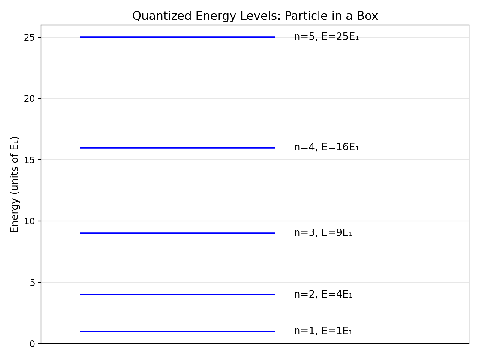
Key insight: Energy is quantized! Only discrete values \(E_1, E_2, E_3, \ldots\) are allowed. The boundary conditions force specific wavelengths, which force specific energies.

What are the wavefunctions?

How do we construct the specific wavefunctions?

From Step 6 above, we found \(k = n\pi/L\) for each quantum number \(n\).

From Step 3, we know the wavefunction has the form:

\[\psi(x) = A \sin(kx)\]

Substitute \(k = n\pi/L\):

\[\psi_n(x) = A \sin\left(\frac{n\pi x}{L}\right)\]

Now we need to determine the normalization constant \(A\).

Finding the normalization constant

The wavefunction must be normalized:

\[\int_0^L |\psi_n(x)|^2 dx = 1\]

Substitute \(\psi_n(x) = A \sin(n\pi x/L)\):

\[A^2 \int_0^L \sin^2\left(\frac{n\pi x}{L}\right) dx = 1\]

Use the identity \(\sin^2(\theta) = \frac{1 - \cos(2\theta)}{2}\):

\[A^2 \int_0^L \frac{1}{2}\left[1 - \cos\left(\frac{2n\pi x}{L}\right)\right] dx = 1\]
\[A^2 \cdot \frac{1}{2} \left[x - \frac{L}{2n\pi}\sin\left(\frac{2n\pi x}{L}\right)\right]_0^L = 1\]

The sine terms vanish at both limits:

\[A^2 \cdot \frac{1}{2} \cdot L = 1\]

Therefore:

\[A = \sqrt{\frac{2}{L}}\]
The complete normalized wavefunctions
\[\boxed{\psi_n(x) = \sqrt{\frac{2}{L}} \sin\left(\frac{n\pi x}{L}\right)} \quad \text{where } n = 1, 2, 3, \ldots\]
Explicit examples for the first few states

Ground state (\(n = 1\)):

\[\psi_1(x) = \sqrt{\frac{2}{L}} \sin\left(\frac{\pi x}{L}\right)\]

This is a sine wave with half a wavelength fitting in the box (one hump).

First excited state (\(n = 2\)):

\[\psi_2(x) = \sqrt{\frac{2}{L}} \sin\left(\frac{2\pi x}{L}\right)\]

This is a sine wave with one full wavelength fitting in the box (two humps, one node at \(x = L/2\)).

Second excited state (\(n = 3\)):

\[\psi_3(x) = \sqrt{\frac{2}{L}} \sin\left(\frac{3\pi x}{L}\right)\]

This is a sine wave with three half wavelengths fitting in the box (three humps, two nodes).

Third excited state (\(n = 4\)):

\[\psi_4(x) = \sqrt{\frac{2}{L}} \sin\left(\frac{4\pi x}{L}\right)\]

This is a sine wave with two full wavelengths fitting in the box (four humps, three nodes).

Pattern summary
  • \(\psi_n(x)\) has \(n\) half-wavelengths in the box

  • \(\psi_n(x)\) has \(n-1\) nodes (points where \(\psi = 0\) inside the box, excluding boundaries)

  • More oscillations → higher \(k\) → higher kinetic energy

  • Each wavefunction satisfies \(\psi_n(0) = \psi_n(L) = 0\) (boundary conditions)

What do these discrete states mean physically?

Are particles always in a single energy state?

Not necessarily! The states \(\psi_1, \psi_2, \psi_3, \ldots\) are called energy eigenstates or stationary states. They have definite energy and their probability distributions don’t change with time.

However, a particle can exist in a superposition of multiple states:

\[\Psi(x,t) = c_1 \psi_1(x) e^{-iE_1 t/\hbar} + c_2 \psi_2(x) e^{-iE_2 t/\hbar} + c_3 \psi_3(x) e^{-iE_3 t/\hbar} + \cdots\]

where \(c_1, c_2, c_3, \ldots\) are complex coefficients satisfying \(|c_1|^2 + |c_2|^2 + |c_3|^2 + \cdots = 1\).

What happens when you measure the energy?

Before measurement: The particle is in a superposition, potentially occupying multiple energy states simultaneously.

During measurement: The wavefunction “collapses” to one of the energy eigenstates.

Measurement result: You always measure one of the discrete energies \(E_1, E_2, E_3, \ldots\), never an in-between value.

Probability: The probability of measuring energy \(E_n\) is \(|c_n|^2\).

Example: Superposition in practice

Suppose a particle is prepared in an equal superposition of the first two states:

\[\Psi(x,t) = \frac{1}{\sqrt{2}} \psi_1(x) e^{-iE_1 t/\hbar} + \frac{1}{\sqrt{2}} \psi_2(x) e^{-iE_2 t/\hbar}\]
What this means:
  • 50% chance of measuring \(E_1 = h^2/(8mL^2)\)

  • 50% chance of measuring \(E_2 = 4h^2/(8mL^2)\)

  • Never measure an energy between \(E_1\) and \(E_2\)

  • The probability density \(|\Psi(x,t)|^2\) oscillates in time (interference between states!)

Why are the energy levels discrete?

The discrete energy levels arise from the boundary conditions. The particle must fit an integer number of half-wavelengths in the box:

\[\lambda_n = \frac{2L}{n}\]

Using de Broglie \(\lambda = h/p\):

\[p_n = \frac{nh}{2L}\]

Only these discrete momenta are allowed, which gives discrete energies:

\[E_n = \frac{p_n^2}{2m} = \frac{n^2 h^2}{8mL^2}\]

Physical intuition: Like a guitar string, only wavelengths that “fit” with the boundary conditions are allowed. The walls enforce standing wave patterns, and standing waves only occur at specific frequencies.

Real-world example: electrons in quantum dots
Quantum dots are tiny semiconductor crystals (nanometers in size) that trap electrons in a small region. The electrons behave like particles in a box, with:
  • Discrete energy levels that depend on the dot size

  • Larger dots → smaller energy spacing (more classical)

  • Smaller dots → larger energy spacing (more quantum)

  • These discrete levels cause quantum dots to emit specific colors of light

(Source code, png, hires.png, pdf)

../_images/plot_particle_in_box.png

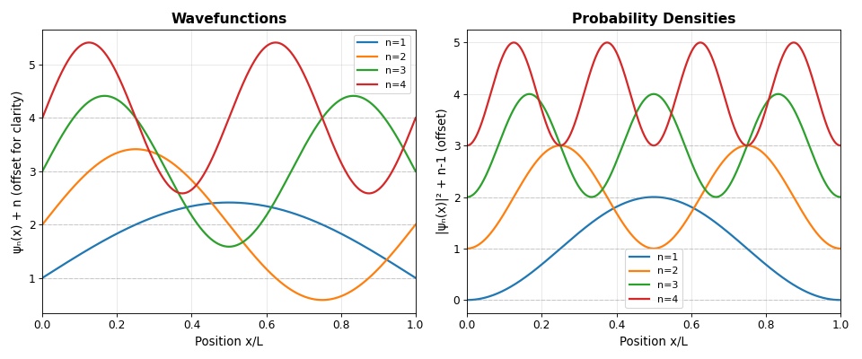
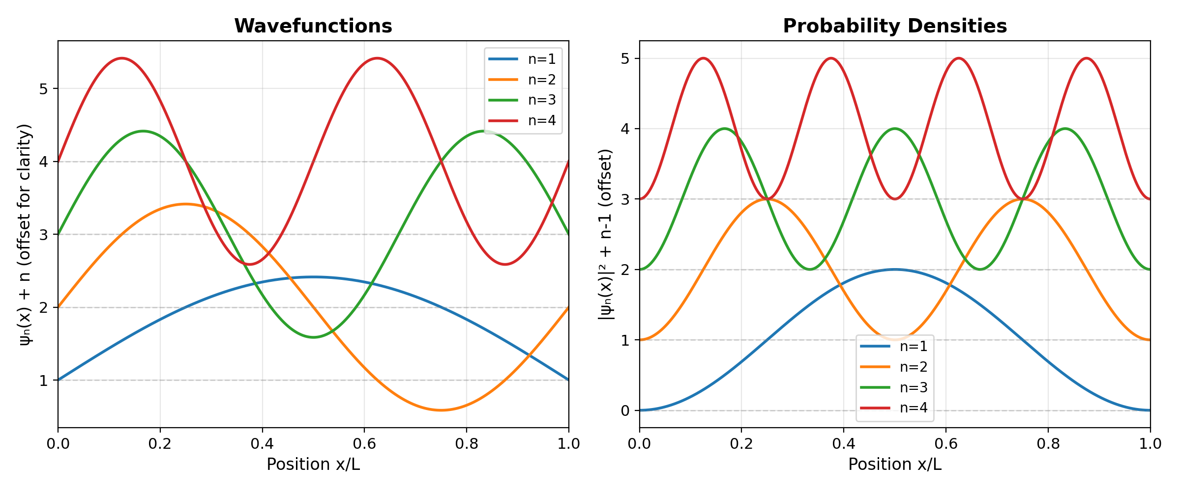
The left panel shows the wavefunctions \(\psi_n(x)\) for the first four quantum states. Each wavefunction has \(n\) half-wavelengths fitting in the box, with \(n-1\) nodes (zero crossings). The right panel shows the probability densities \(|\psi_n(x)|^2\), indicating where the particle is most likely to be found. For the ground state (\(n=1\)), the particle is most probable at the center. Higher energy states show multiple peaks and nodes.

Energy level spacing

The energy difference between consecutive levels:

\[E_{n+1} - E_n = \frac{\pi^2 \hbar^2}{2mL^2}[(n+1)^2 - n^2] = \frac{\pi^2 \hbar^2}{2mL^2}(2n + 1)\]
Key observations:
  • Spacing increases with \(n\) (not equally spaced!)

  • Smaller box → larger spacing (quantum effects more pronounced)

  • Heavier particle → smaller spacing (more classical behavior)

Energy level diagram

(Source code, png, hires.png, pdf)

../_images/plot_particle_in_box_energy_levels.png

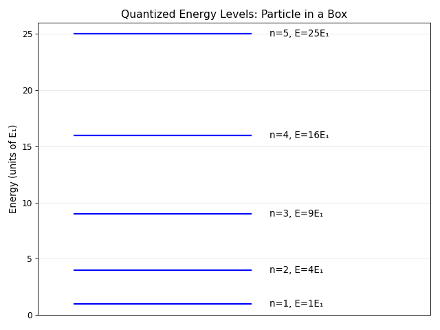
The energy levels \(E_n = n^2 E_1\) are shown as horizontal blue lines, where \(E_1 = h^2/(8mL^2)\) is the ground state energy. Notice how the spacing between levels increases with quantum number \(n\): the spacing grows as \(E_{n+1} - E_n = (2n+1)E_1\). This increasing spacing is a key difference from the harmonic oscillator, which has constant spacing.

Why is energy quantized?

Standing wave condition: Only wavelengths that fit an integer number of half-wavelengths in the box are allowed:

\[L = n \frac{\lambda}{2} \quad \Rightarrow \quad \lambda = \frac{2L}{n}\]
Why must the waves fit within the box boundaries?

The particle cannot exist outside the box because \(V = \infty\) in those regions. The wavefunction must be zero at \(x = 0\) and \(x = L\) (boundary conditions).

This means we can only have standing waves that:
  • Start at zero: \(\psi(0) = 0\)

  • End at zero: \(\psi(L) = 0\)

  • Have an integer number of half-wavelengths between the walls

Just like a guitar string fixed at both ends, only certain wavelengths “fit” in the box. Wavelengths that don’t satisfy the boundary conditions would create destructive interference and cannot exist as stable states.

(Source code, png, hires.png, pdf)

../_images/plot_standing_waves_in_box.png
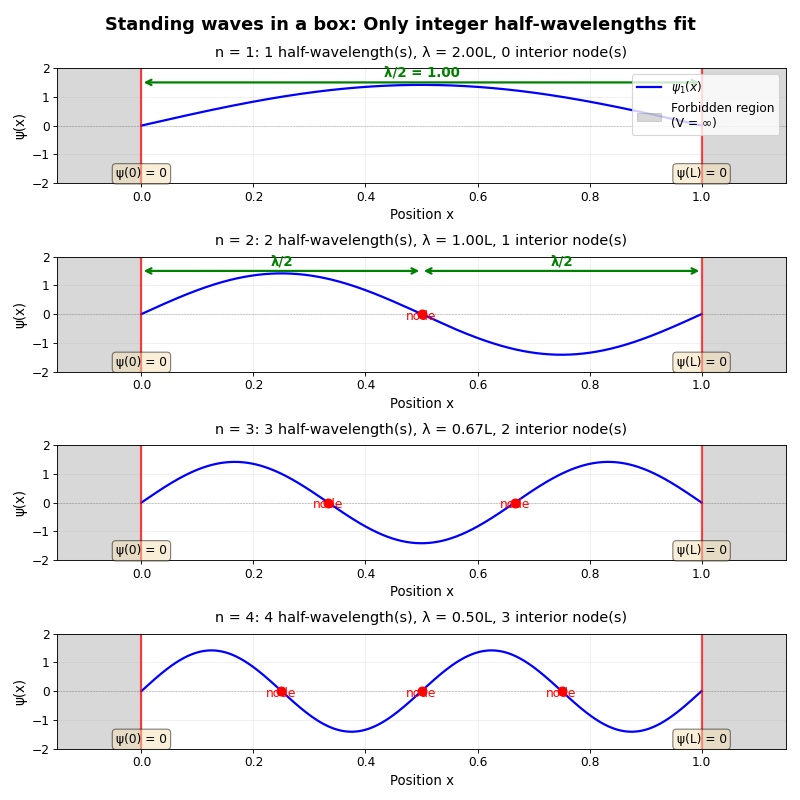
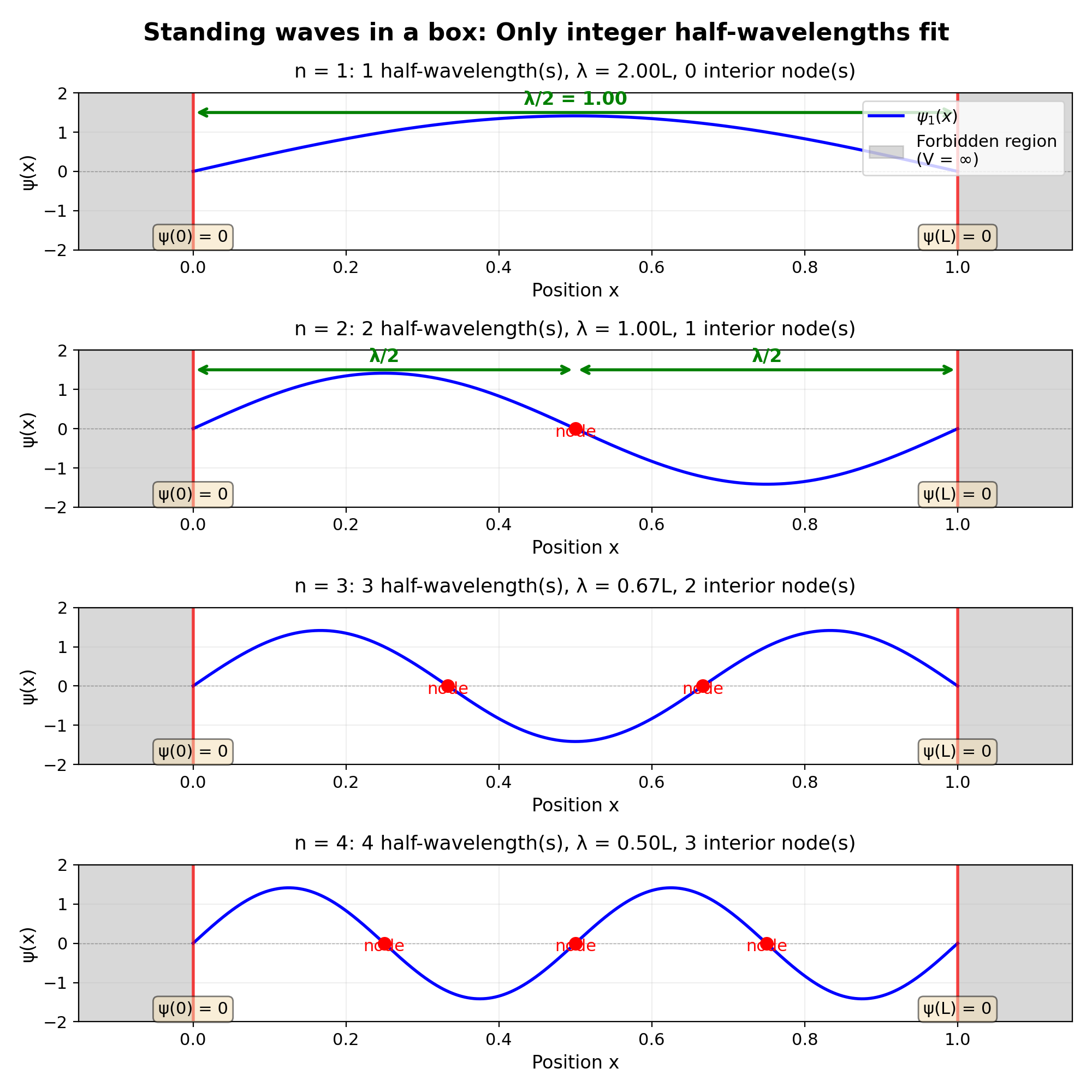
The figure above shows the first four standing wave patterns. Notice:
  • Each wavefunction goes to zero at the walls (\(x=0\) and \(x=L\))—required by boundary conditions

  • Gray shaded regions show the forbidden regions where \(V=\infty\) (particle cannot exist there)

  • \(n=1\): one half-wavelength fits in the box

  • \(n=2\): two half-wavelengths (one full wavelength) fit in the box

  • \(n=3\): three half-wavelengths fit in the box

  • \(n=4\): four half-wavelengths (two full wavelengths) fit in the box

  • Red dots mark nodes (places where \(\psi=0\) inside the box)

How does this lead to discrete energies?

Using de Broglie (\(\lambda = h/p\)) and \(E = p^2/(2m)\):

\[p = \frac{h}{\lambda} = \frac{nh}{2L}\]
\[E = \frac{p^2}{2m} = \frac{n^2 h^2}{8mL^2}\]

Physical intuition: Like a guitar string, only certain “notes” (energies) are allowed. The box imposes boundary conditions that select discrete wavelengths, which correspond to discrete momenta and therefore discrete energies.

An interesting observation: Mass doesn’t appear in the wavefunction

Wait, there’s no mass in \(\psi_n(x) = \sqrt{2/L} \sin(n\pi x/L)\)?
That’s right! The normalized wavefunction depends only on:
  • The box size \(L\)

  • The quantum number \(n\)

  • Position \(x\)

The mass \(m\) does not appear in the wavefunction itself.

Where does mass matter then?

Mass appears in the energies, not the wavefunctions:

\[E_n = \frac{n^2 h^2}{8mL^2}\]
Heavier particle (\(m\) large):
  • Lower energy levels (energies scale as \(1/m\))

  • Same wavefunctions (same spatial patterns)

  • Smaller de Broglie wavelength at same energy

Lighter particle (\(m\) small):
  • Higher energy levels

  • Same wavefunctions

  • Larger de Broglie wavelength at same energy

Why is this interesting?

This reveals a deep fact about quantum mechanics: The spatial structure of allowed states depends only on the boundary conditions (geometry), not on what particle is in the box.

  • An electron and a proton in the same box have identical wavefunction shapes

  • But the proton’s energy levels are ~2000 times lower (because \(m_{\text{proton}} \approx 2000 \, m_{\text{electron}}\))

  • The probability distributions \(|\psi_n(x)|^2\) are identical regardless of particle mass

Physical meaning: The wavefunction describes where the particle can be found (geometry). The energy describes how fast it’s moving (kinetics). Mass couples the two through \(E = p^2/(2m)\), but doesn’t change the allowed spatial patterns.

What about the “shape” of the electron?

In quantum mechanics, elementary particles like electrons are treated as point particles—they have no internal structure or “shape” in the classical sense.

The wavefunction \(\psi(x)\) doesn’t describe the electron’s shape; it describes the probability of finding the electron at different locations. The electron itself is a point, but its probability distribution is spread out according to \(|\psi(x)|^2\).

This is fundamentally different from classical physics, where we might imagine a tiny ball bouncing around. In quantum mechanics:
  • The electron doesn’t have a trajectory

  • It doesn’t have a definite position until measured

  • \(|\psi(x)|^2\) tells us the probability density, not the electron’s “size” or “shape”

Next steps

Continue to Quantum mechanics II for advanced topics including quantum harmonic oscillator, perturbation theory, and relativistic quantum mechanics.