Theme 1A & 1B: Spot size and convergence angle (Talos)
Caution
VERY ROUGH DRAFT, NOT AUTHORITATIVE. Week 3 of the Stanford MATSCI 322 TEM Lab, taught by Andrew Barnum, Pinaki Mukherjee, and Ash. Recorded on 2026-04-21, with an additional underfocus/overfocus session on 2026-04-23. Photos, notes, data, and analysis captured by @bobleesj (Sangjoon Bob Lee) during the sessions as a student. Terminology, step ordering, and values may be wrong or incomplete. Treat this page as a personal study reference, not an SOP. A trained user must verify everything before relying on it.
This lab addresses the following questions:
- How do the spot-size knob and the C2 aperture shape the beam that hits the sample (Theme 1A)?
- How does the C2 lens switch the illumination between parallel, convergent, and defocused, and how does that choice distinguish image mode from diffraction mode (Theme 1B)?
Each section below opens with the specific sub-questions it tackles, then walks through the experiment, the data, and the answer.
Links:
- SNSF Talos reservation / info page: TODO
- Thermo Fisher Talos L120C product page: TODO
System specifications (observed):
| Model | Talos (Thermo Fisher) |
| Accelerating voltage | 120 kV (session value; instrument also supports others) |
| Camera | BM-Ceta |
| C2 apertures tested | 70 µm, 50 µm (handout also lists 150 µm, 100 µm) |
| Probe modes | Microprobe (used in this session), Nanoprobe |
| Magnification range observed | 5,300× (imaging) to 45,000× (for Theme 1B convergent work) |
Acronyms:
C1: first condenser lens (spot-size lens)C2: second condenser lens (intensity / illumination lens)SA: selected areaCL: camera lengthDP: diffraction patternTIA: TEM Imaging and Analysis (Thermo Fisher software)mulXY: multifunction X/Y knobs on the hand panelR1,R3,L3: buttons on the hand control pad (R1 raises/lowers the fluorescent screen; R3 / L3 step spot size up / down)
Overview
| Theme | What you study | Output |
|---|---|---|
| 1A: Beam parameters | Spot size 1–11 × two C2 apertures; record C1, C2, screen current, camera length | Data tables, plots, convergence-angle analysis for lab report |
| 1B: C2 lens & illumination for diffraction | Parallel vs convergent vs defocused beam on oriented gold; lens values in image vs diffraction mode | Lens-value table, C2-condition table, ray diagram sketch |
Theme 1A: How do spot size and C2 aperture shape the beam?
What this section addresses
The beam that reaches the sample is the product of two things: the condenser lens system (C1 sets the spot size, C2 sets the illumination) and the condenser aperture selection. Three sub-questions to answer:
- When the spot-size knob is stepped, what actually moves? Only C1? Or C2 as well?
- The intensity knob clearly moves C2. Does it move C1 too?
- How much does the aperture change matter? Is a 70 µm aperture really that different from 50 µm at the same spot size?
Diffraction camera length for a 5 mm beam
| Spot size | CL at 70 µm C2 | CL at 50 µm C2 |
|---|---|---|
| 3 | 1.75 m | 2.2 m |
| 9 | 1.75 m | 2.21 m (recovered from Ceta .emd metadata; not measured directly with the 5 mm marking) |
Plots

What did the data tell us?
- Spot size drives C1, not C2. C1 swings from ~17% at spot 1 to ~93% at spot 11, a factor of 5. C2 drifts from ~44.5% to ~39%, only about 5 percentage points.
- The aperture barely moves the lenses. The 70 µm and 50 µm curves sit on top of each other in both C1 and C2 plots. The aperture clips the beam; it doesn’t reshape the lens system.
- The intensity knob moves C2 but not C1 (confirmed by watching the System Status panel while turning intensity).
- Screen current drops by ~200× from spot 1 to spot 9 at fixed aperture (5.80 nA → 0.030 nA on the 70 µm curve), approximately exponential on the log-y plot (about a factor of two per step).
- 70 µm delivers ~2× the screen current of 50 µm at every spot above the detection limit. The area ratio is (70/50)² ≈ 2, which matches: the aperture really is just clipping.
- A 5 mm beam needs longer camera length at 50 µm C2. At spot 3: 1.75 m (70 µm) vs 2.2 m (50 µm). Less beam, so more camera length is needed to magnify it to the same ring.
How big is the convergence angle, and what sets it?
In diffraction mode the focused-probe central disk has angular radius equal to α. With the disk set to fill the inner 5 mm screen marking (small-angle limit, α = 2.5 mm / L):
| C2 aperture | Spot | Camera length L | α = 2.5 mm / L |
|---|---|---|---|
| 70 µm | 3 | 1.75 m | 1.43 mrad |
| 70 µm | 9 | 1.75 m | 1.43 mrad |
| 50 µm | 3 | 2.20 m | 1.14 mrad |
| 50 µm | 9 | 2.21 m | 1.13 mrad |
The result. α is set by the C2 aperture, not by spot size. At a given aperture, α is the same at spot 3 and spot 9. Going from 70 µm to 50 µm at spot 3 reduces α from 1.43 to 1.14 mrad. The 50 µm aperture clips the convergent cone to a smaller half-angle.
Why doesn’t spot size affect α? (ray diagram)
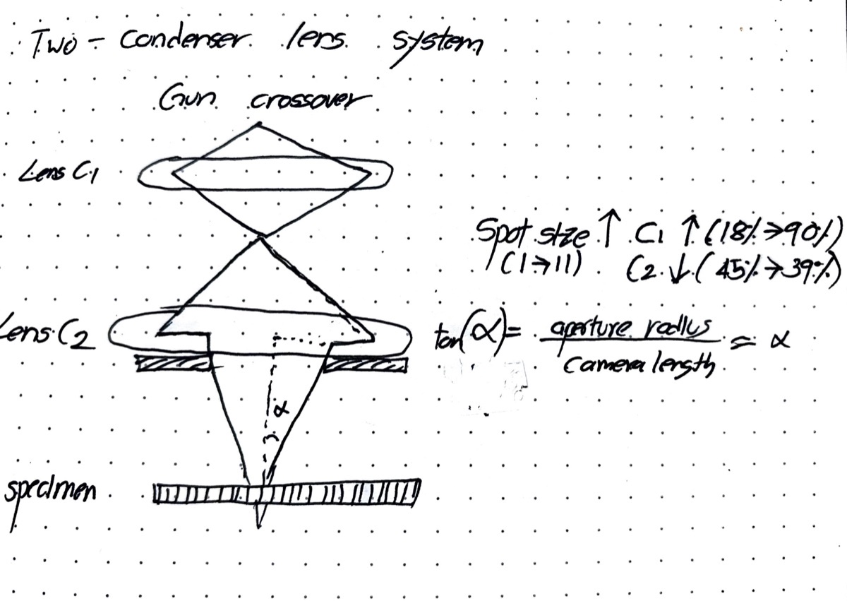
The electron beam travels down the column in this order: it starts at the gun crossover, passes through the C1 lens, forms an intermediate crossover, gets clipped by the C2 aperture, passes through the C2 lens, and lands on the specimen.
The spot-size knob only changes how strongly C1 is excited. Turning C1 up shortens its focal length, which shrinks the image of the gun crossover that arrives at the C2 aperture. A more shrunken crossover means a smaller, dimmer probe on the specimen.
What the spot size cannot change is the C2 aperture radius (r_ap). The aperture is a physical disk with a fixed hole, so it always clips the converging cone to the same radius. C2 then projects that cone onto the specimen at a fixed distance away. Putting these two together: the convergence half-angle α at the specimen is set by the aperture radius and that fixed C2-to-specimen distance, and is independent of the spot size. In the small-angle limit, tan(α) ≈ α = r_ap / L.
Why is C1 so low at spot 1?
Spot 1 wants the largest probe and the highest current, which means the least demagnification of the gun crossover. C1 at minimum strength does the least demagnification, hence the very low percentage at spot 1. As the spot number increases, more demagnification is requested, so C1 % climbs.
Why does one camera length cover both spot 3 and spot 9?
The 5 mm-beam method sets the focused-probe central disk equal to the 5 mm screen ring. Disk radius = α × L. Because α is fixed by the C2 aperture (independent of spot size), a single L gives the 5 mm condition for every spot at that aperture. The 50 µm aperture has a smaller α, so a larger L (2.2 m vs 1.75 m) is needed to inflate its disk back to 5 mm.
Theme 1B: How does the C2 lens switch between parallel and convergent illumination?
What this section addresses
Theme 1A focused on the beam at crossover. But the beam has more states than that: it can be parallel, convergent to a point, or defocused on either side of crossover. Each state changes what the sample sees, and the switch between image mode and diffraction mode on a TEM is really just a choice of which lenses are doing what.
Two sub-questions to answer:
- When the instrument switches between imaging and diffraction modes, which lenses actually change values? Is it really a C2 thing, or do the post-sample lenses do the heavy lifting?
- What does the beam at the sample look like when defocused clockwise vs counter-clockwise through crossover? Are the two sides symmetric, or does something meaningful change?
The sample is a commercially-available oriented gold standard: evaporated to ~11 nm, (100) orientation, loaded in a double-tilt holder and aligned to its zone axis before the session started.
Experimental setup
Two sub-experiments.
Experiment 1: lens values in image vs diffraction mode. At 5,300× magnification with C2 = 70 µm and spot size 9, the beam is expanded clockwise through crossover until the diffraction pattern becomes sharp (parallel illumination). The four post-sample lens values (Diffraction, Intermediate, Projector 1, Projector 2) are recorded from the System Status panel in image mode, then again after switching to diffraction mode with CL = 420 mm.
Experiment 2: sweeping through crossover. Camera length is increased to 2.2 m and magnification to 45,000×. The beam is focused to a point on the phosphor, and the central disk is centered with mulXY. The intensity knob is then turned clockwise from the focused point until features reappear inside the central disk; next, counter-clockwise through crossover and past it until features reappear on the other side. An image is acquired at each stopping point, along with the C2 value.
Note: if the phosphor screen “flaps” when
R1is pressed, press again until it settles in the desired position. This is normal instrument behavior.
Which lenses change between image mode and diffraction mode?
| Lens | Image mode (%) | Diffraction mode (%) |
|---|---|---|
| Diffraction | 44.65 | 28.42 |
| Intermediate | -14.81 | -0.281 |
| Projector 1 | 41.81 | 52.84 |
| Projector 2 | 97.09 | 98.07 |
How does the beam change as C2 is swept through crossover?
The successive states the beam passes through during Experiment 2, read top to bottom along the C2 knob:
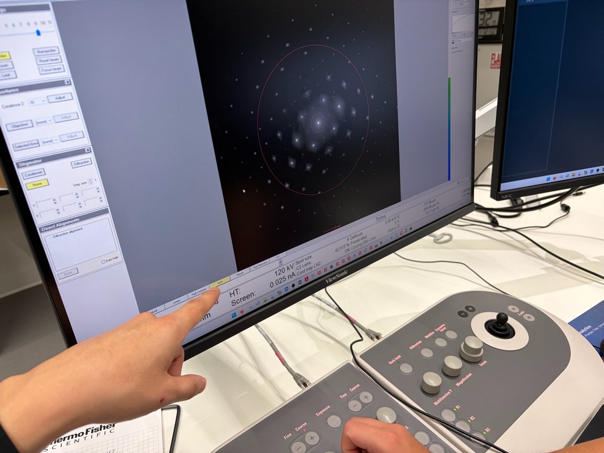
- Parallel (start): beam expanded post-crossover, diffraction pattern sharp, C2 = 42.01%.
- Convergent (at crossover): C2 turned clockwise into crossover so the beam focuses to a point on the phosphor. Central disk is featureless with only a few scattered spots. This is the reference point for the defocus sweep.
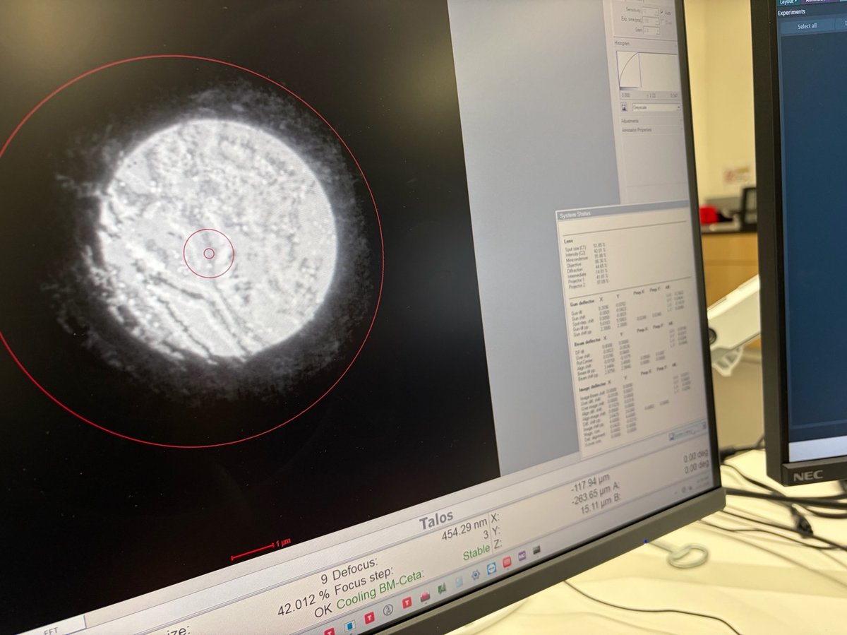
- Defocused clockwise from focus: from crossover, C2 is nudged further clockwise (slightly stronger) until features reappear inside the central disk. C2 = 40.06%, beam diameter ≈ 1.28 µm.
- Back through focus, then defocused counter-clockwise: C2 is rotated counter-clockwise past crossover until features appear again. C2 = 38.663%, beam diameter ≈ 1.39 µm. Features look the same as in step 3, but the real-space orientation is flipped.
The full table with FluCam image-mode and diffraction-mode captures for each of these conditions is in the FluCam screenshots section below.
The C2 values for steps 3 and 4 straddle the crossover value (39.396%) by roughly ±0.7 percentage points in either direction. The ~0.7% offset is how far the intensity knob had to travel past crossover before the central disk showed features again.
What did the data tell us?
- Switching image to diffraction mode moves every post-sample lens, with the Intermediate lens doing the actual mode switch. Diffraction lens 44.65 → 28.42%, Intermediate −14.81 → −0.281%, Projector 1 41.81 → 52.84%, Projector 2 essentially unchanged. The full mechanism is in the Ray diagrams section below.
- C2 values for each beam condition are close but not identical. Parallel at 5,300× is C2 = 42.01%. Convergent (beam focused to a point) at 45,000× is C2 = 39.396%. Defocused on either side of crossover is ±1% around the crossover value.
- Defocus clockwise and counter-clockwise through crossover produce images that look the same, but are flipped in real space. Past crossover, the beam inverts: features you saw on the left end up on the right.
- Short camera length = wider diffraction view; long camera length = tighter central disk. At 350 mm CL many Bragg peaks fit on screen; at 2.2 m CL only the central disk and nearest reflections fit.
- Thermo Fisher’s mental model: the beam is the reference point. Start from parallel illumination in image mode; watching how the beam converges or diverges as you adjust C2 is how you reason about every other mode.
How do the same lenses produce both an image and a diffraction pattern?
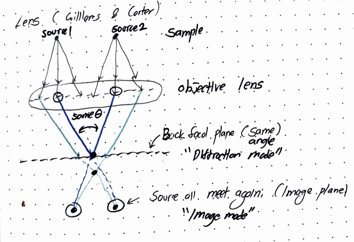
Two sample sources emit fans of parallel-illumination rays. The objective lens has two natural conjugate planes downstream:
- At the back focal plane, rays of the same exit angle (regardless of which source they came from) focus to one point. That is the diffraction pattern.
- At the image plane (further down), rays from the same source (regardless of exit angle) focus to one point. That is the real-space image.
The objective is unchanged between the two modes; what switches is the intermediate lens, which re-focuses the camera onto either the back focal plane (diffraction mode) or the image plane (image mode). The lens-excitation table above shows this directly: the intermediate lens swings from −14.81% to −0.281% while the objective stays put.
The “Diffraction lens” name is misleading. It is the first projection lens after the objective, not a lens that is only on in diffraction mode. It actually gets weaker in diffraction mode (44.65% → 28.42%) because once the intermediate lens drops out, Projector 1 takes over and gets stronger; the chain has one fewer stage to do work, so the Diffraction lens slackens.
Does Bragg’s law agree with the displayed camera length?
The Ceta .emd files carry the full FEI metadata (acceleration voltage, camera length, lens excitations, pixel scale). For the Ceta diffraction acquisitions taken in this session: HT = 120 kV, spot index = 9, C1 = 51.85% (matching the 50 µm aperture spot 9 row of the data table), camera lengths = 2.209 m (#0015–17) and 1.065 m (#0018–21). The 70 µm aperture was not used during the Ceta diffraction acquisitions.
Relativistic wavelength (λ = h·c / √(eV·(eV + 2 m_e c²))):
| HT | λ (pm) |
|---|---|
| 120 kV (this session) | 3.35 |
| 200 kV | 2.51 |
| 300 kV | 1.97 |
Bragg angle for gold {200} (d_200 = a/2 = 0.2035 nm; small-angle: 2θ_B ≈ λ/d):
| HT | 2θ_B for {200} (mrad) |
|---|---|
| 120 kV | 16.5 |
| 200 kV | 12.3 |
| 300 kV | 9.7 |
True camera length from the {200} reflection. Using the Velox pixel scale (0.01628 1/nm/pixel for L = 1.065 m), the {200} spot lies at q = 1/d_200 = 4.91 1/nm, which is 4.91 / 0.01628 = 302 pixels from the central beam. With effective pixel size 56 µm, this is 302 × 56 µm = 16.9 mm. Then L_true = 16.9 mm / 16.5 mrad = 1.024 m. For #0015–17 the same calibration gives L_true ≈ 2.221 m.
Comparison of displayed vs metadata vs Bragg-back-calculated camera length:
| Capture | L displayed (m) | L from .emd metadata (m) | L calculated from {200} Bragg (m) | Agreement |
|---|---|---|---|---|
| #0015–17 | 2.20 | 2.209 | 2.221 | within 1% |
| #0018–21 | 1.05 | 1.065 | 1.024 | within 4% |
All three agree within ~4%, which is the expected calibration accuracy for the Talos camera-length setting.
True convergence angle. The 5 mm-marking measurement on the 50 µm aperture was made at L = 2.20 m, so the matching Bragg-calibrated camera length is L_true = 2.221 m (from #0015–17). Then α_true = 2.5 mm / 2221 mm ≈ 1.13 mrad, in agreement with the screen-marking value of 1.14 mrad to within 1%.
What is the effective Ceta pixel size at 120 kV vs 300 kV?
The Ceta has 14 µm physical pixels. With binning 4 the output frame is 1024 × 1024 with effective pixel = 56 µm. The real-space pixel size at the specimen depends on imaging mode (microprobe vs nanoprobe) and magnification, not on HT directly: HT only changes the wavelength (and therefore the reciprocal-space pixel scale in diffraction mode). For the Ceta in diffraction mode at L = 1.065 m:
- At 120 kV (λ = 3.35 pm), reciprocal pixel = 56 µm / (1065 mm × 0.00335 nm) = 0.0157 1/nm/px. Velox-reported pixel scale: 0.01628 1/nm/px (3.7% disagreement, consistent with the camera-length calibration above).
- At 300 kV (λ = 1.97 pm), reciprocal pixel = 56 µm / (1065 mm × 0.00197 nm) = 0.0267 1/nm/px (predicted; not measured this session).
Higher kV covers more reciprocal space per pixel at the same camera length (each pixel spans more 1/nm), so more Bragg orders fit in the camera FOV, at the cost of coarser q resolution per pixel.
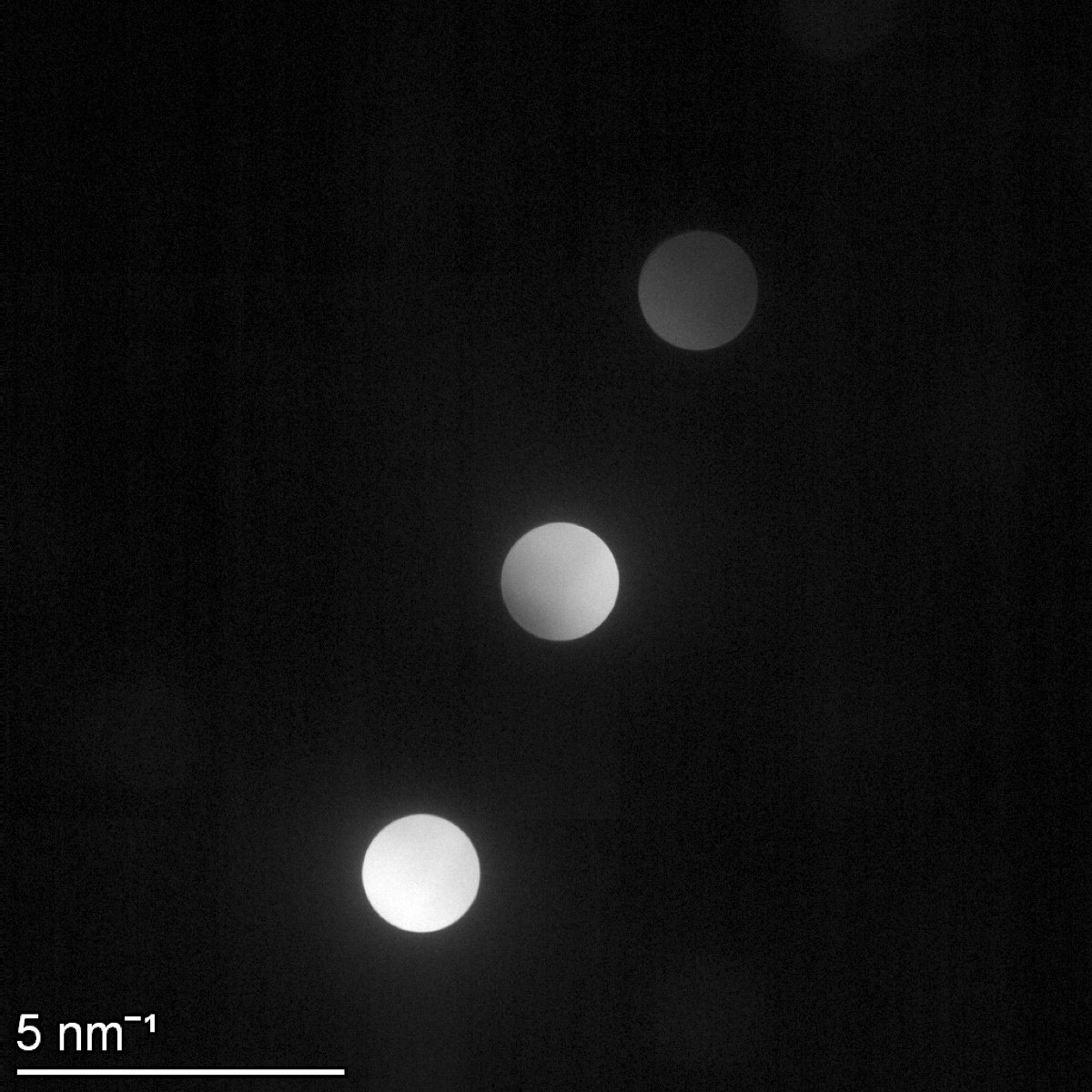
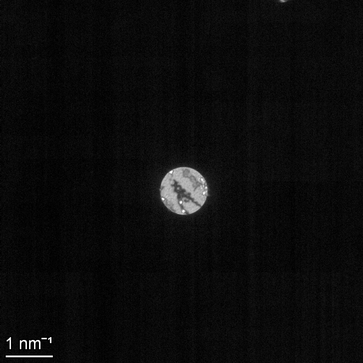
Why does longer camera length show fewer Bragg spots?
Camera length in a TEM behaves like the throw distance of a movie projector:
- Move the projector close to the wall (short L): the image on the wall is small, but the whole picture fits.
- Move the projector far from the wall (long L): the image on the wall is huge, but only the center fits in view.
Diffraction mode works the same way. Every Bragg spot sits at a fixed angle 2θ from the center; on the camera it lands at r_on_camera = 2θ × L.
- Long L (2.20 m): each Bragg spot is far from center, the pattern is spread out, and the fixed-size camera only catches the central disk plus maybe one reflection (Ceta capture below at 1 nm⁻¹ scale).
- Short L (1.05 m): spots land closer to center, more spots squeeze inside the camera, and the gold (100) zone-axis spots start to appear (Ceta capture below at 5 nm⁻¹ scale).
- Very short L (350 mm, observed in 1B but not recorded with the Ceta): many Bragg orders fit at once, ideal for whole-pattern overviews.
So long L means “magnify reciprocal space” (good for measuring α from the central disk against a screen marking); short L means “wide-angle reciprocal view” (good for seeing the whole pattern at once).
| L = 2.20 m (focused central disk) | L = 1.05 m (focused central disk with gold {200} spots in view) |
|---|---|
 |
 |
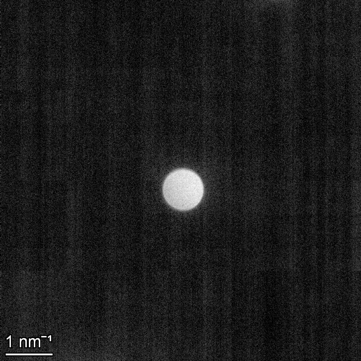
Can the over- vs under-focus flip be seen directly on the Ceta?
The two Ceta captures below were taken at L = 2.20 m on opposite sides of the focused crossover. The diagonal dark band inside the disk shifts/inverts between the two, while the outer disk geometry (set by the C2 aperture) is unchanged. This is the over/under-focus contrast inversion (sign change in the contrast transfer function), shown here in the central disk itself rather than in the real-space image.
| L = 2.20 m, defocused side A (#0016) | L = 2.20 m, defocused side B (#0017) |
|---|---|
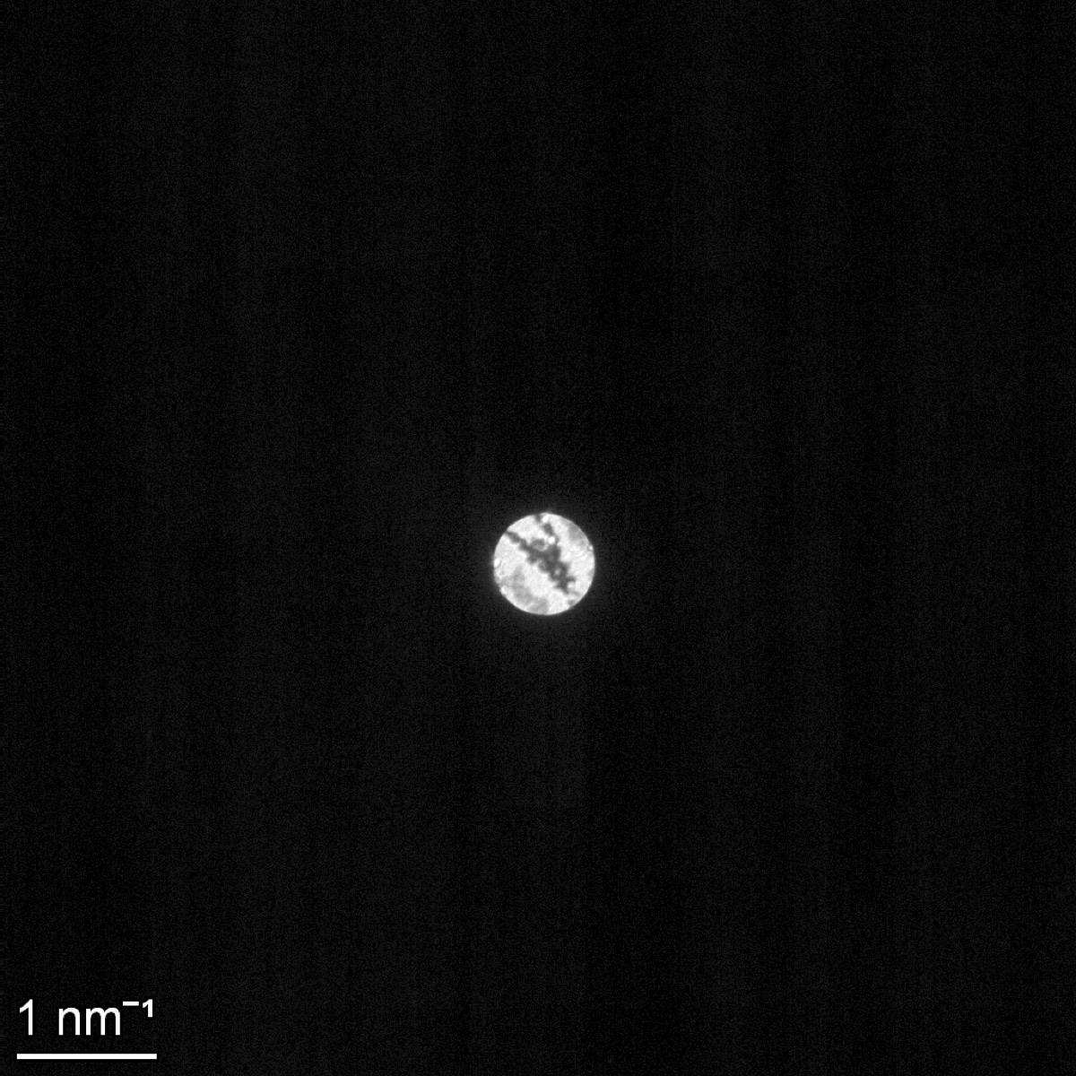 |
 |
What does each C2 condition look like on the FluCam?
The four C2 conditions from the lab table mapped to the FluCam captures (image mode and diffraction mode for each). Image/diffraction mode classification comes from the .emi ObjectInfo (Real Space vs Reciprocal Space); the four conditions were mapped to the eight tifs by combining the timestamp order of the .emi files (procedure flow: Parallel → Convergent → Defocused #1 → Defocused #2) with the visible scale bar and probe geometry in each tif. The Parallel and Convergent assignments are unambiguous from the beam diameter; the Defocused #1 vs #2 pairing is inferred from chronological order (the per-tif .ser metadata was not in the folder).
| C2 condition | Mag | C2 (%) | Beam diameter | Camera length | Image mode (FluCam) | Diffraction mode (FluCam) |
|---|---|---|---|---|---|---|
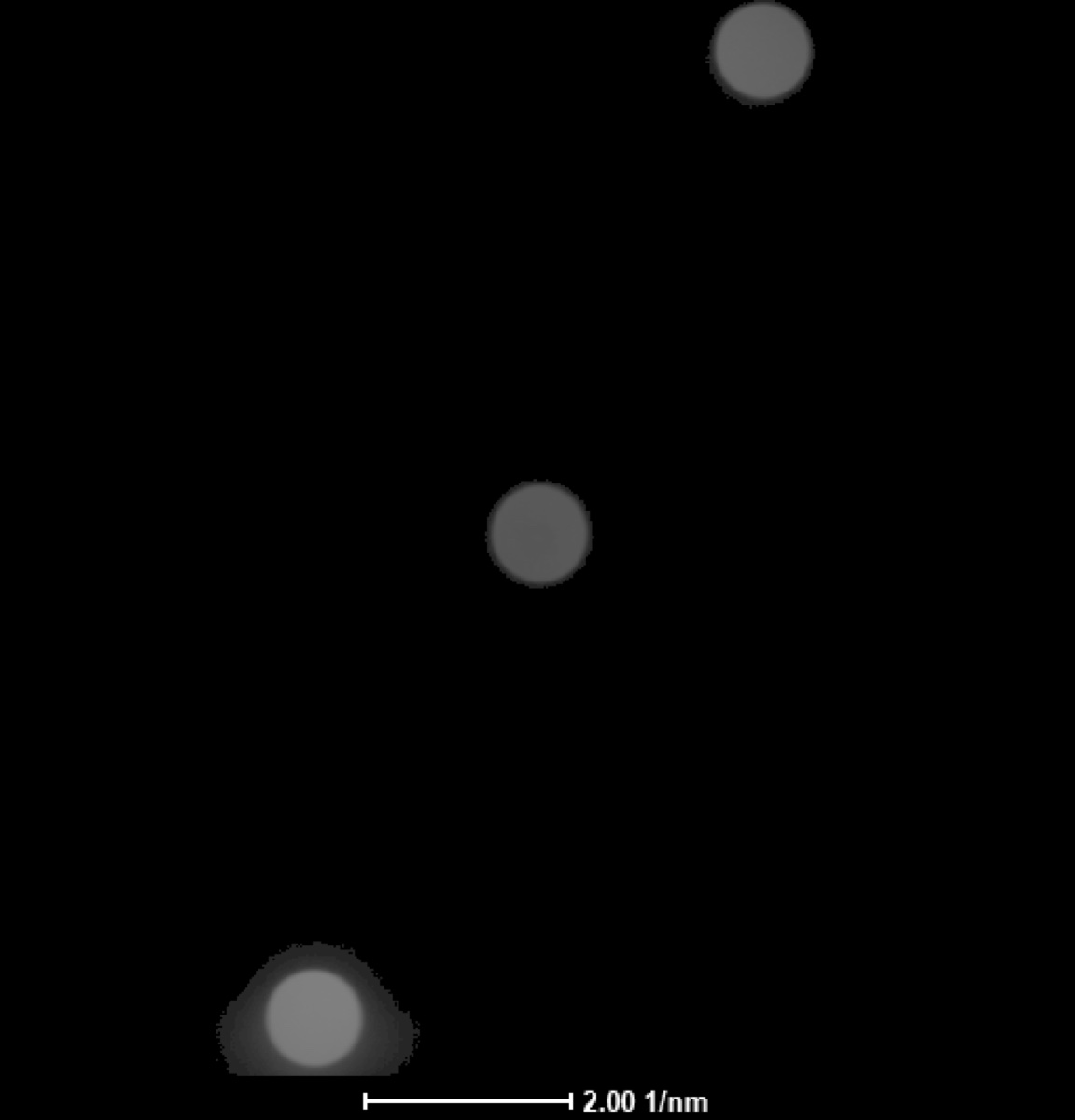
| Parallel | 5,300× | 42.01 | 5.25 µm | 420 mm |  tif 3 · 2 µm scale |
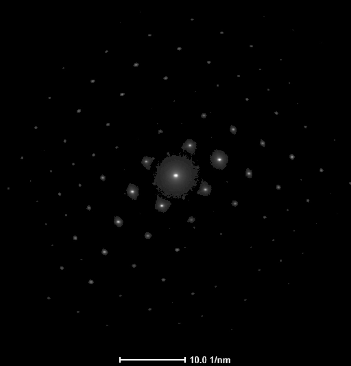 tif 2 · 10.0 1/nm |
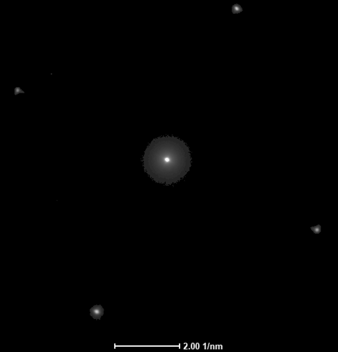
| Convergent (focused crossover) | 45,000× | 39.396 | 73 nm | 2.2 m | 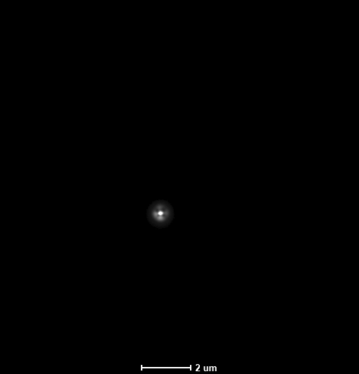 tif 8 · 2 µm scale |
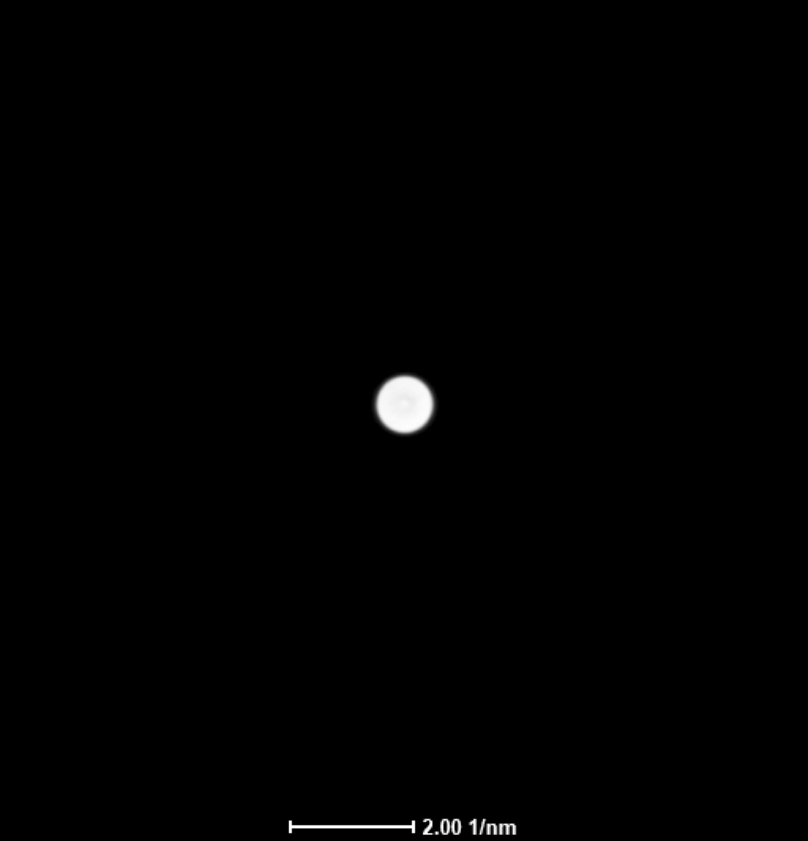 tif 1 · 2.00 1/nm |
| Defocused #1 (intensity knob clockwise from convergent, C2 up) | 45,000× | 40.06 | 1.28 µm | 2.2 m | 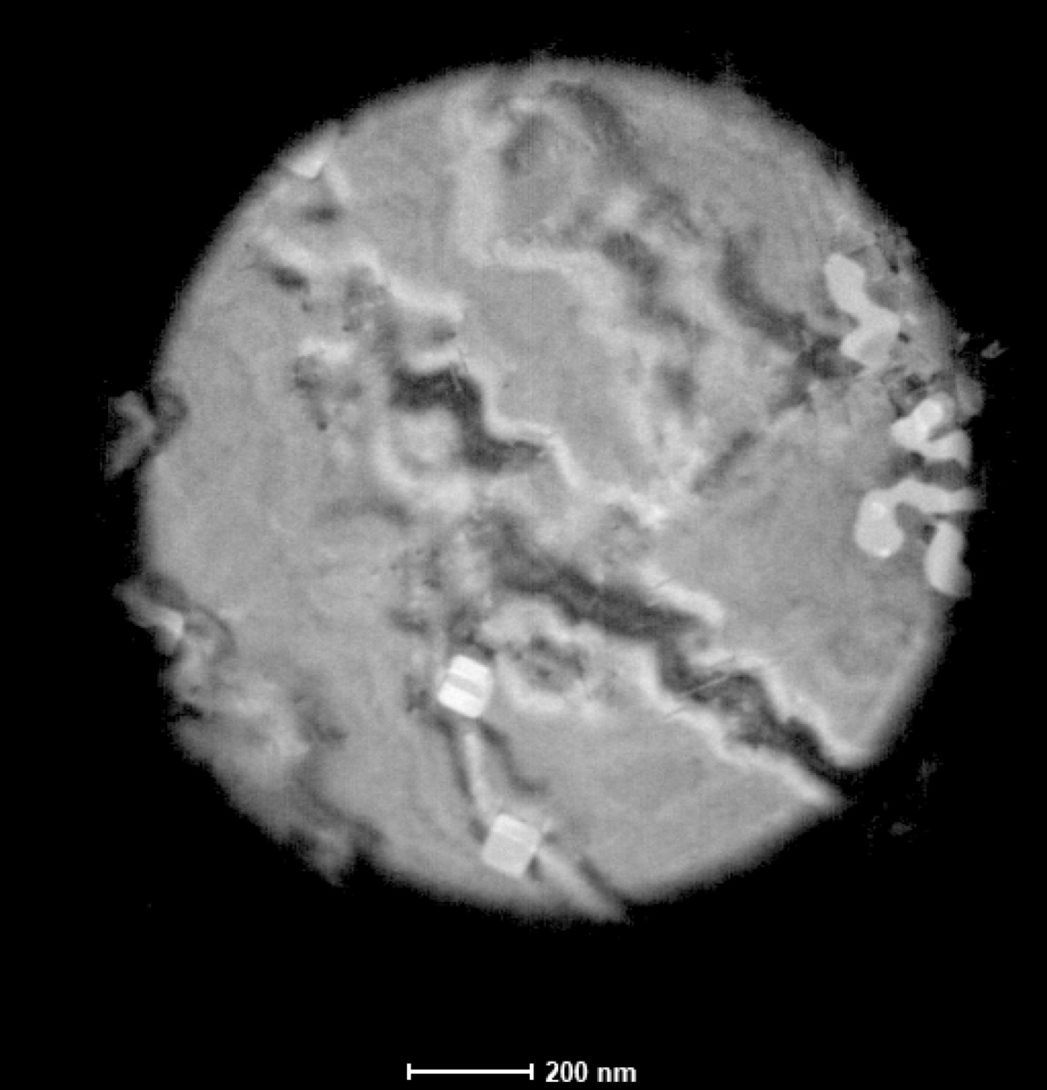 tif 6 · 200 nm scale |
 tif 4 · 2.00 1/nm |
| Defocused #2 (intensity knob counter-clockwise from convergent, C2 down) | 45,000× | 38.663 | 1.39 µm | 2.2 m | 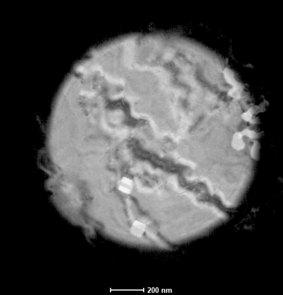 tif 7 · 200 nm scale |
 tif 5 · 2.00 1/nm |
Stepping through Defocused #1 → Convergent → Defocused #2 sweeps the intensity knob through the focused crossover. The two defocused image-mode probes (tif 6 vs tif 7) cover the same sample area but show inverted internal contrast; the two defocused diffraction-mode disks (tif 4 vs tif 5) similarly flip their internal fringes. Whether the “C2 up” side corresponds to true overfocus or underfocus depends on whether the C2-lens perspective or the beam perspective is being used (these conventions are opposite).
Why does the image flip when defocus crosses zero?
When the beam crossover sits above the sample plane (over-focus), the rays have already crossed by the time they reach the sample, so left/right is inverted on the specimen. When the crossover sits below the sample plane (under-focus), the rays have not crossed yet, so the orientation is preserved. Stepping the intensity knob through crossover swaps over- and under-focus, hence the real-space flip.
Changelog
- May 11, 2026 : Filled in the Theme 1A and Theme 1B analysis (convergence angle, two-condenser ray diagram, Williams and Carter ray diagram, Bragg’s law verification of camera length, comparison to displayed and
.emdmetadata values, effective real-space pixel calculation). Recovered the spot 9 / 50 µm camera length from the Ceta.emdmetadata. Added a brief reference to the over/under-focus session of 2026-04-23. - Apr 22, 2026 : Initial draft from the 2026-04-21 Week 3 TEM class lab taught by Andrew B. Photos, notes, and measurements by @bobleesj. Plots generated from the xlsx data sheet. Analysis prompts and ray diagrams left as TODO for the lab report.