Electron Microscopy (WIP)
Step-by-step visual guides for learning TEM. Focused on practice sitting in front of the microscope with visual elements.
WIP:
- Use real screenshots instead of pictures
- Better pictures: proportion, focus, FOV
- More visuals added to each session when needed
Disclaimer: Always follow https://barnum.su.domains/ for correctness. Only use this documentation if you are working with the authors and need quick visual references.
Available guides
| Guide | Instrument | Description | Readiness | Status |
|---|---|---|---|---|
| STEM (Spectra) | Spectra | STEM probe correction and imaging | 8/10 | Available |
| TEM (Spectra) | Spectra | Optional TEM alignment and image correction | 5/10 | Available |
| TEM (Titan) | Titan | TEM alignment and imaging | - | Coming soon |
| 4DSTEM | Spectra | 4DSTEM with Dectris detector | 4/10 | Available |
| EELS | Spectra | Electron Energy Loss Spectroscopy | 2/10 | Available |
| EDS | Spectra | Energy Dispersive X-ray Spectroscopy | 2/10 | Available |
| Aberration Correction (Advanced) | Spectra | Manual aberration correction without Sherpa | 1/10 | Available |
| Phenom Pharos (Deep Lab) | Phenom Pharos G2 | Desktop SEM/STEM operation guide | 2/10 | Available |
| Spot size and convergence angle | Talos | Class lab on beam parameters and C2 illumination | 3/10 | Available |
| Drop casting | : | Grid preparation by drop casting nanoparticles | 2/10 | Available |
| Tomography | Spectra | Electron tomography | - | Coming soon |
| Ptychography | Spectra | Ptychography imaging | - | Coming soon |
| MAPED | Spectra | Precession Electron Diffraction | - | Coming soon |
Instrument links:
Other resources:
Looking for volunteers!
We appreciate feedback, corrections, and contributions from the community!
- Found an error? Open an issue or submit a PR
- Want to add your institution’s SOP? Reach out to @bobleesj — we can help with writing and formatting as long as you have notes, Word docs, or rough drafts
- Have suggestions? See the GitHub repo for contribution guidelines
Acknowledgments
Authors thank Dr. Pinaki Mukherjee and Andrew Barnum for training @bobleesj and Guoliang Hu at Stanford SNSF.
Changelog
- Apr 22, 2026 - Reorganize sidebar into SNSF Spectra 300, Techniques, Class labs, Grid preparation, Sample loading sections
- Apr 22, 2026 - Add class lab guide on spot size and convergence angle (Talos)
- Apr 22, 2026 - Add drop casting grid preparation guide
- Mar 1, 2026 - Restructure STEM and TEM guides, add pre-session checklist and end session procedures
- Feb 28, 2026 - Reorganize guide structure, rename directories, add safety warnings
- Jan 31, 2026 - Add STEM probe correction guide with screenshots from Andrew Barnum training
- Jan 31, 2026 - Add draft Titan TEM guide
- Dec 18, 2025 - Add EELS and EDS guides
- Dec 17, 2025 - Use mdBook to render static pages and host on GitHub
- Dec 14, 2025 - Begin Electron Microscopy training documentation, led by @bobleesj
TEM (Spectra)
This guide covers optional TEM alignment on the Spectra 300: column setup, eucentric height, aperture alignment, and image correction. TEM mode is useful for fast sample navigation and for users who need TEM-specific data (HRTEM, diffraction patterns). Most users will proceed directly to STEM (Spectra).
Prerequisite: The sample is already loaded and the holder is inserted into the Spectra 300. For sample loading and end session procedures, see STEM (Spectra).
Acronyms:
mulXY- Multifunction X/Y knobs on hand panelTEMUI- TEM User Interface (software)
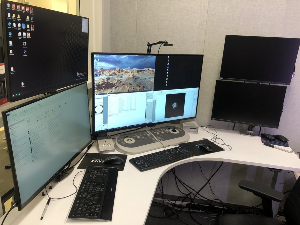
Workstation layout:
| Monitor | Software | Purpose |
|---|---|---|
| Bottom left | TEMUI | Microscope control, vacuum, alignments |
| Bottom right | Velox | Live imaging, acquisition |
| Top left | ImageCorrector | Aberration measurement & correction |
| Top right | Velox image gallery | Captured images from Velox |
Overview
This guide covers two main phases:
| Phase | Procedures | Time |
|---|---|---|
| Part 1: Column alignment | Vacuum check, beam setup, eucentric height, monochromator, C2 aperture, condenser stigmatism, beam tilt, rotation center | 10-15 min |
| Part 2: Image correction | Capture image, C1A1 correction, Tableau measurement, save settings | 10-15 min |
Part 0: Safety check
Complete the pre-session checklist in STEM (Spectra) before proceeding. Do not skip this step.
Part 1: Column alignment
1.1 Open column valves
Before imaging, verify that the vacuum system is ready and the column valves can be safely opened.
-
Verify vacuum pressure
-
In
TEMUI, check the vacuum pressure values on the log scale (lower = better):Gauge Log Value Why Important Gun 1 Highest vacuum needed for stable electron emission Liner <10 Prevents electron scattering along beam path Octagon 1 Protects sample from contamination and oxidation Projection <30 Maintains image quality in projection system Buffer tank <50 Ensures stable pumping performance Backing line <80 Turbo pump pushes compressed gas into the backing line
-
-
Open column valves
-
In
TEMUI, clickCol Valves Open. The status changes to indicate the column valves are open and the turbo pump is off.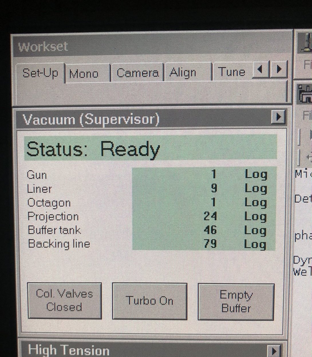
-
-
Set condenser apertures
-
In
TEMUI, go to theTunetab, thenApertures. Set Condenser 1, 2, 3 to 2000, 70, 1000.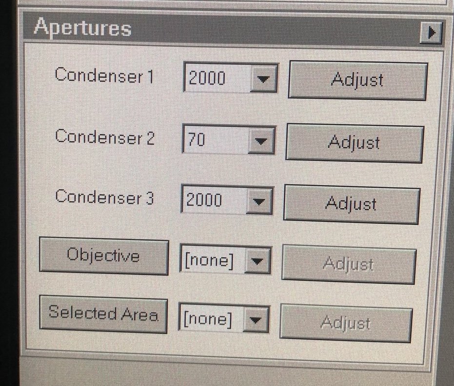
-
1.2 Beam setup
Configure the beam parameters for initial navigation and sample finding.
-
Enter TEM mode
- On the
Veloxsoftware (bottom right monitor), verify TEM mode is active. If not, click theTEMbutton.
- On the
-
Set spot size
- Set Spot Size 3 by pressing the
L3orR3button on the hand panel. As spot size decreases, screen current increases and the image gets brighter. - If the image is too bright, turn the intensity knob to decrease the screen current to around 2 nA and press
Linearmode to see better contrast.
- Set Spot Size 3 by pressing the
-
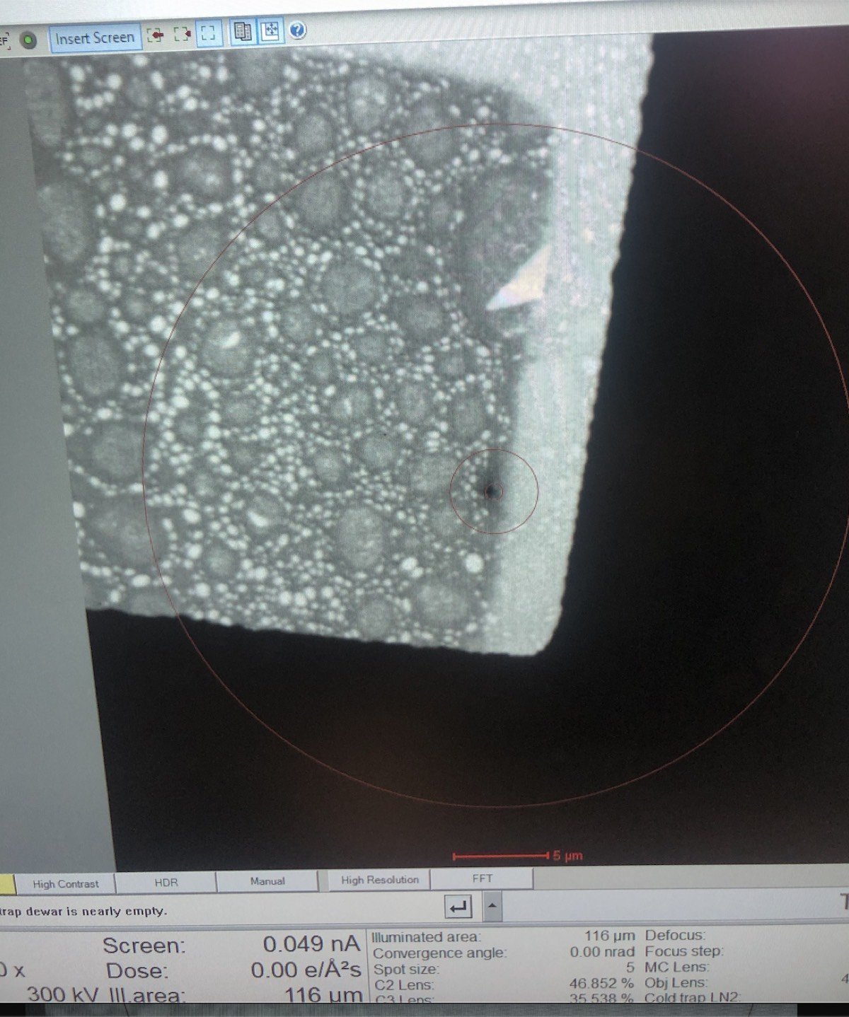
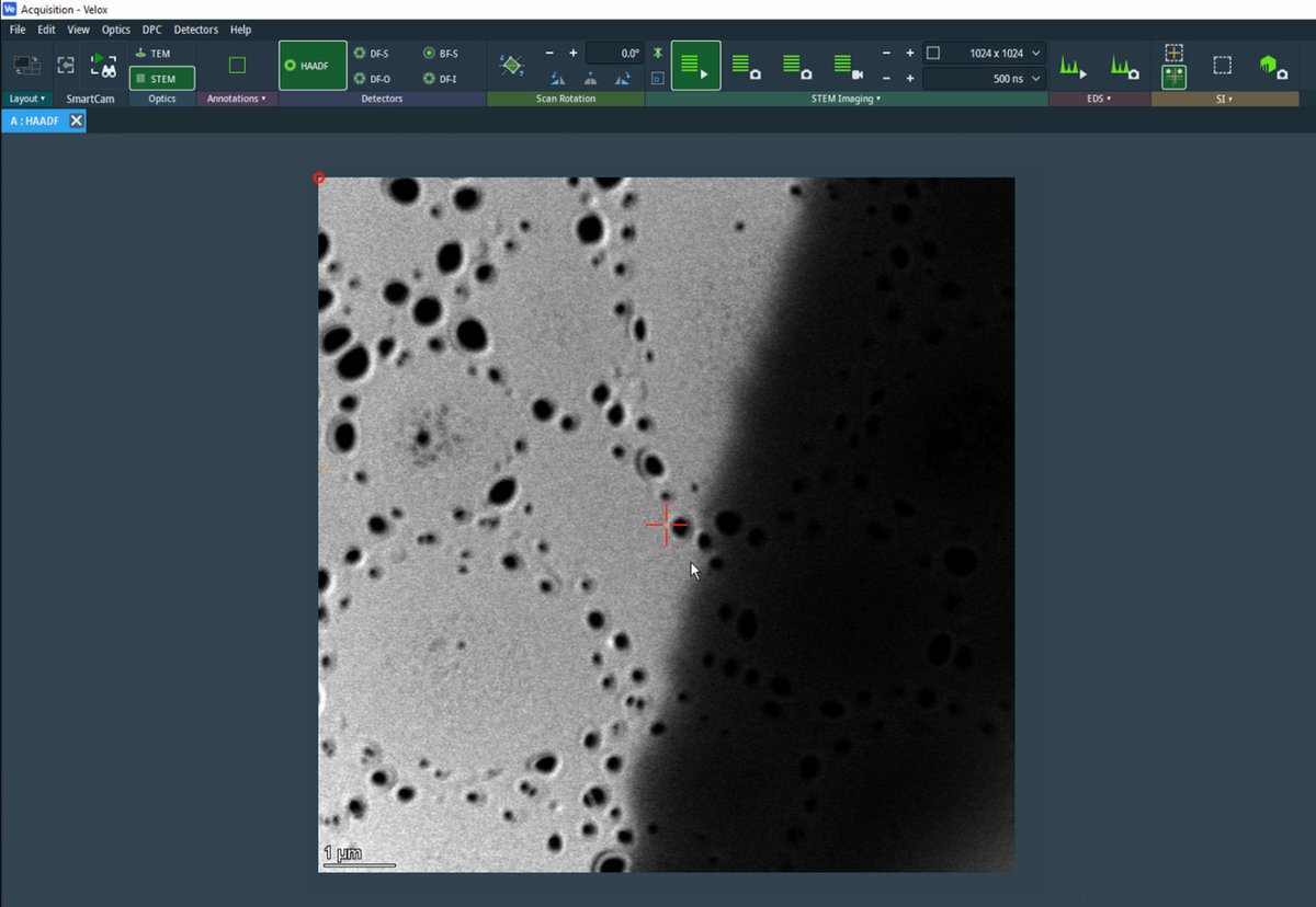
Find sample region
-
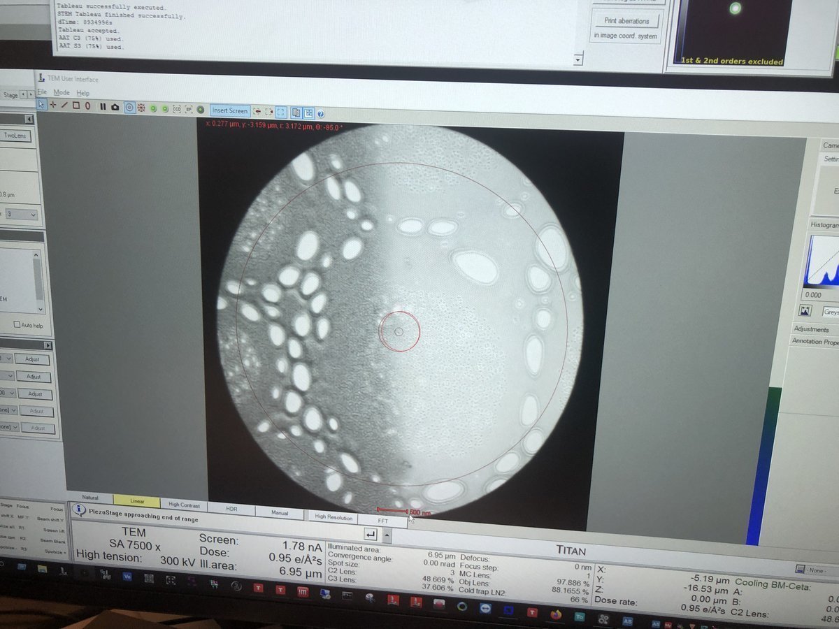
Set ~500x magnification by adjusting the magnification knob.
-
Locate the gold (dark) and amorphous carbon boundary by driving the joystick on the hand panel. This contrast boundary serves as a visual marker to identify the region of interest across various magnifications.
-
1.3 Eucentric height
At eucentric height, the sample remains stationary when tilted. This is essential for accurate imaging and aberration correction. Complete eucentric height alignment after loading each sample. Do not skip this step.
-
Adjust z-axis
-
Set ~7,500x magnification by adjusting the magnification knob.
-
Press
z-axisup or down on the hand panel. Watch the image contrast change as the sample moves through focus. At eucentric height, the contrast is minimized (the image appears most “washed out”).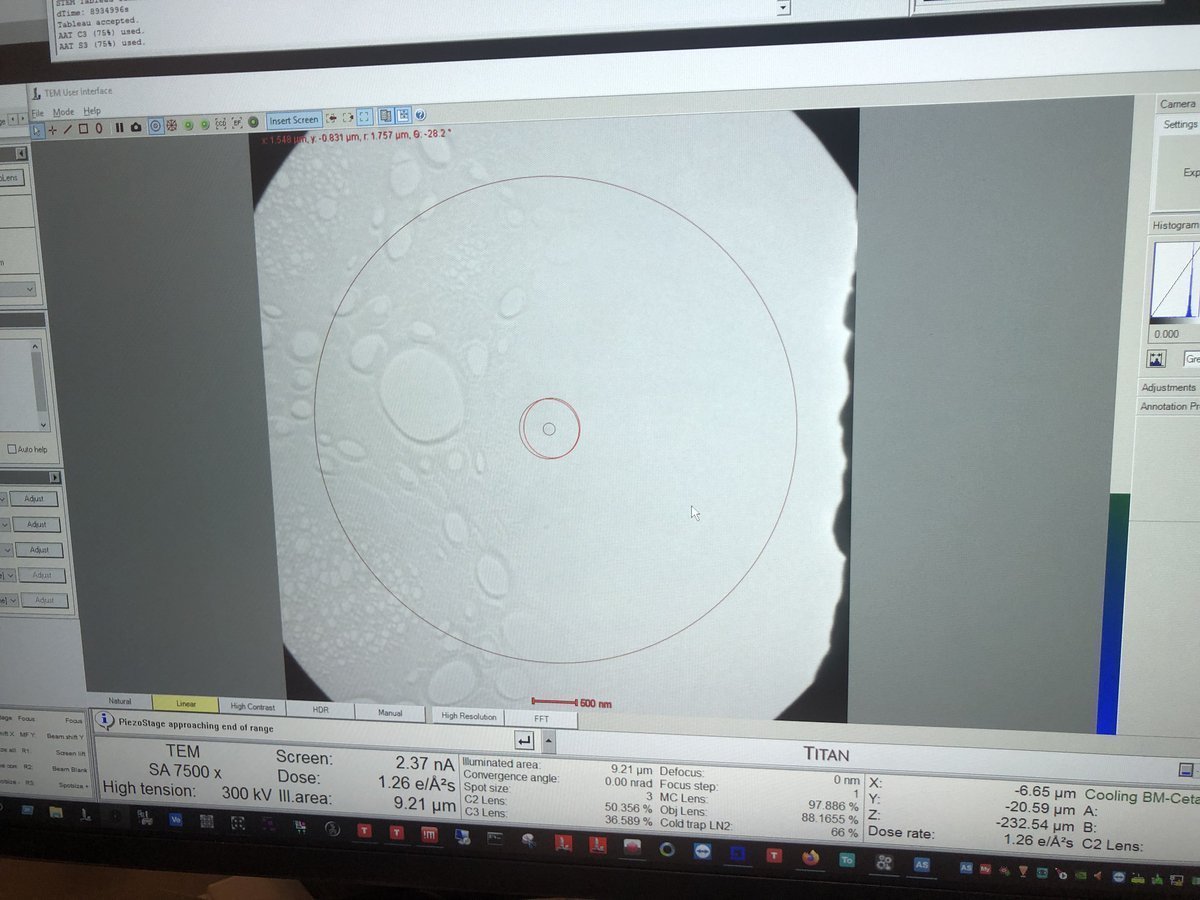
-
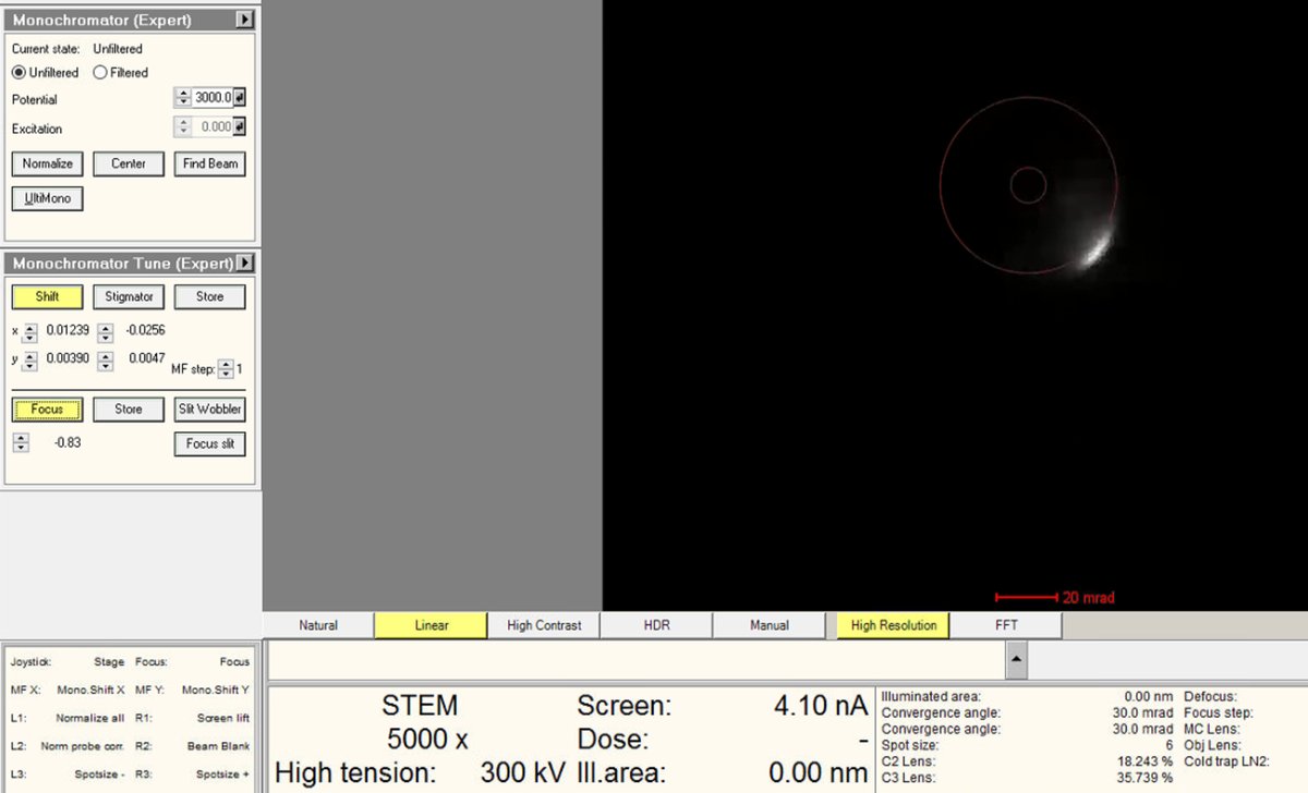
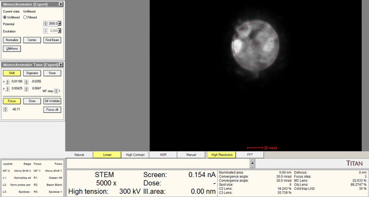
1.4 Monochromator tune
The monochromator selects a narrow energy range from the electron beam. If the beam edge looks jagged, the monochromator needs alignment.
-
Check beam edge
- Do you see a jagged area along the beam edge in the previous step? If not, skip this section. Otherwise, follow the steps below.
-
Adjust monochromator
-
In
TEMUI, go to theMonotab, then openMonochromator Tune (Expert)and clickShift.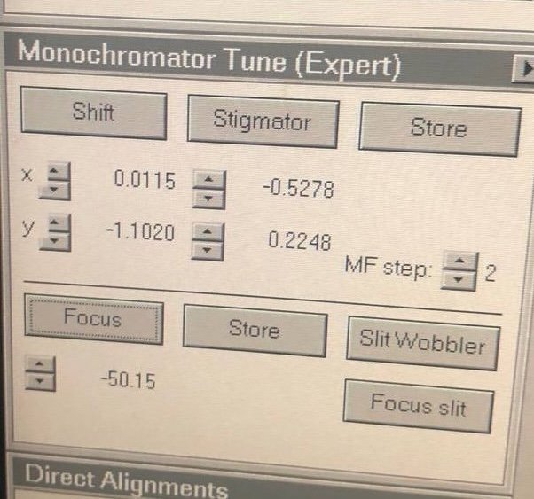
-
Adjust
mulXYknobs until the jagged area disappears.
-
1.5 C2 aperture alignment
The C2 aperture controls convergence angle and beam size. It blocks off-axis electrons — only electrons within a certain angular range pass through. A user must center this aperture on the optical axis so that the beam expands and contracts symmetrically.
-
Enter two-lens mode
-
In
TEMUI, go to theTunetab, thenBeam Settings, and clickTwolens. In two-lens mode, C3 is turned off, so the beam behavior on screen is purely from C2. This makes it straightforward to detect and correct any C2 aperture misalignment. In three-lens mode, C3 reshapes the beam after C2, masking the misalignment.
-
-
Center and align C2 aperture
-
Center the beam by rolling the hand panel ball.
-
Converge the beam by varying the intensity knob.
-
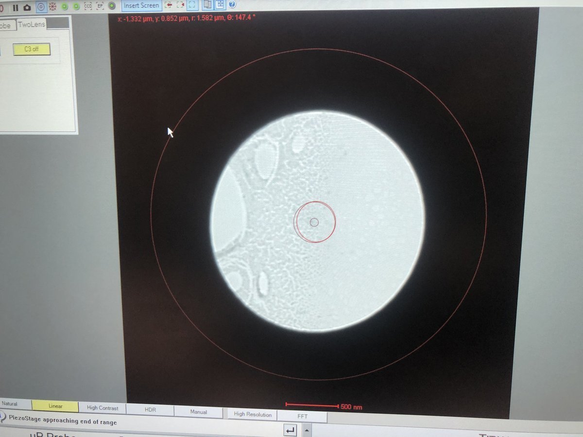
Vary beam size by turning the intensity knob counterclockwise and clockwise. Notice the beam expansion is not concentric — this indicates the C2 aperture is off-center.
-
Make the beam concentric: go to
Apertures, clickAdjustnext toCondenser 2, then adjust themulXYknobs until the beam expands and contracts concentrically.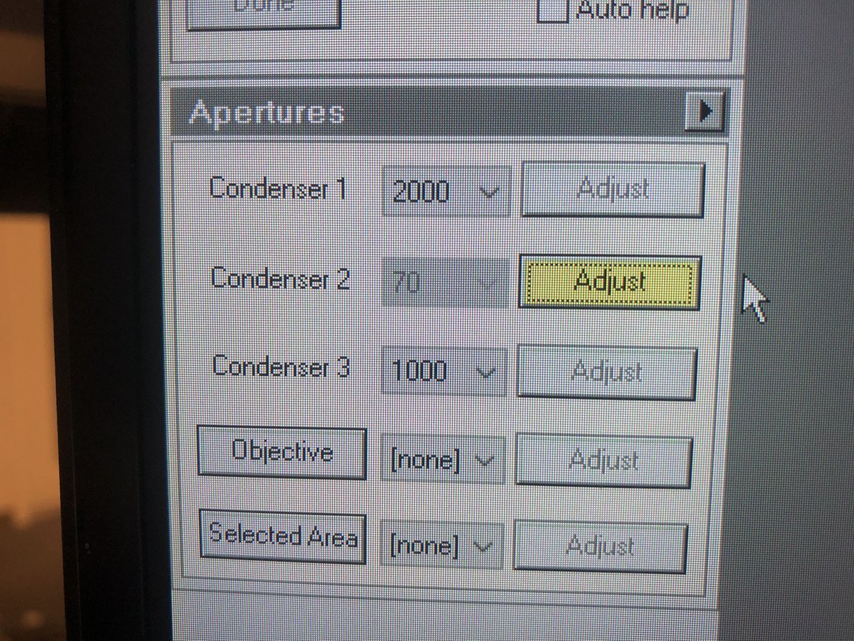
-
-
Return to three-lens mode
-
In
TEMUI, go toBeam Settingsand clickTEMto return to three-lens mode.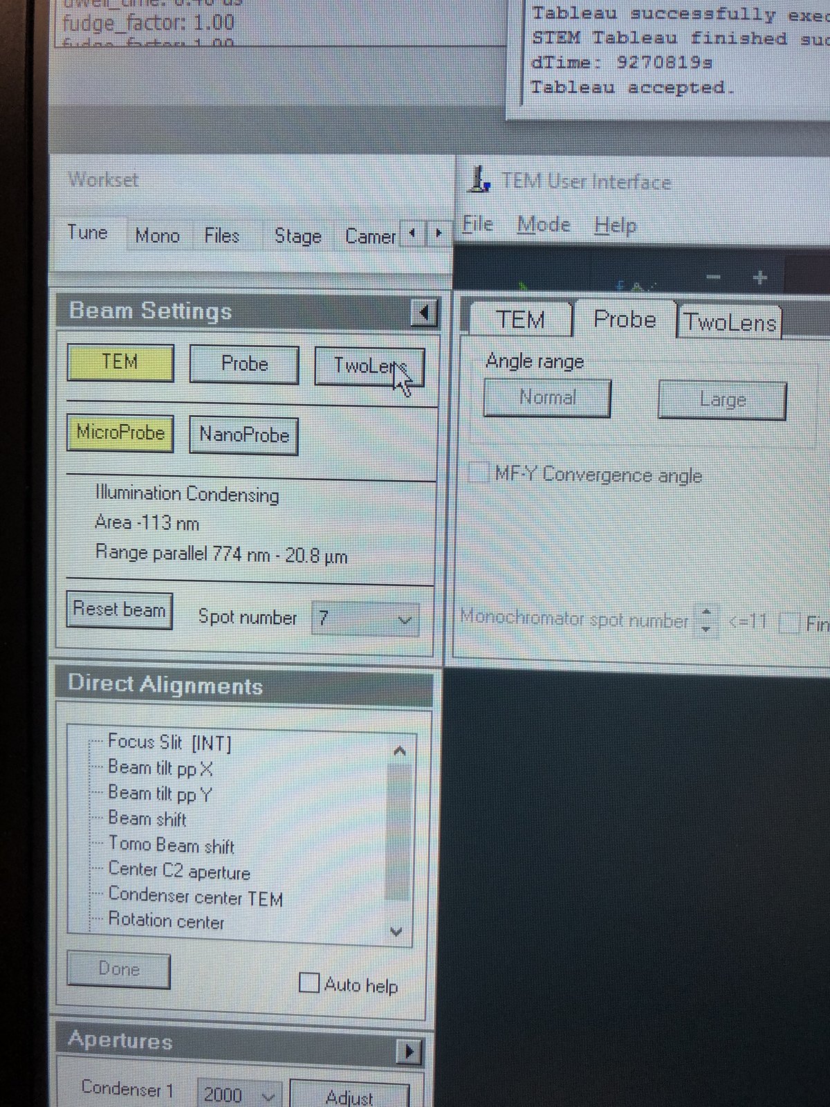
-
Verify the beam is centered and concentric.
-
1.6 Condenser stigmatism
Condenser astigmatism causes the beam to appear elliptical instead of round. Correcting this ensures a symmetric probe.
-
Increase magnification
- Set ~200kx magnification by adjusting the magnification knob.
- If the beam has shifted from center, go to
Tunetab, thenDirect Alignment, clickBeam Shift, and adjust themulXYknobs to re-center.
-
Correct stigmatism
-
Enlarge the beam by adjusting the intensity knob.
-
In
TEMUI, clickStigmator, thenCondenser. Adjust themulXYknobs to make the beam as round as possible. The beam should remain circular as you vary the intensity knob. PressNonewhen done.
-
1.7 Beam tilt
Beam tilt alignment minimizes lateral beam shift when the beam angle changes. Proper alignment ensures the beam tilts around a single point without drifting.
-
Align beam tilt
- In
TEMUI, go toDirect Alignmentand clickBeam tilt pp X. Adjust themulXYknobs to minimize the lateral jiggle. - Repeat for
Beam tilt pp Y. - If the beam center has shifted, click
Beam Shiftand adjust themulXYknobs to re-center.
- In
1.8 Rotation center
Rotation center alignment ensures the image rotates around the center of the field of view when focus changes.
-
Align rotation center
- In
TEMUI, go toDirect Alignmentand clickRotation Center. The image pulses in and out of focus. - Adjust the
mulXYknobs to minimize lateral movement. The pulsing should appear concentric (expanding and contracting from the same point) with no side-to-side drift.
- In
Part 2: Image correction
2.1 Capture image
Before running the image corrector, a user must set up live imaging in Velox and find a suitable sample region.
-
Prepare for imaging
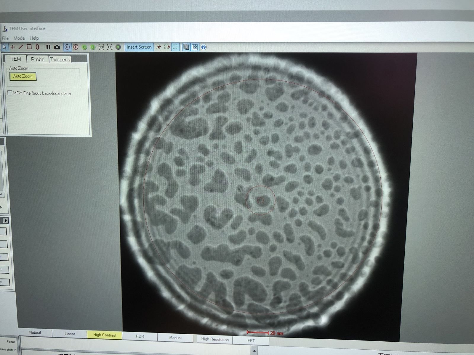
- Find a flat area with a distribution of particle sizes and no holes.
- Important: Enlarge the beam to cover the entire fluorescent screen before lifting it. When the screen is raised, the camera and detectors below are exposed to the beam. A concentrated beam can permanently damage them.
- Press
R1on the hand panel to lift the fluorescent screen.
-
Start live imaging
-
In
Velox(right monitor), click the play button to start live imaging.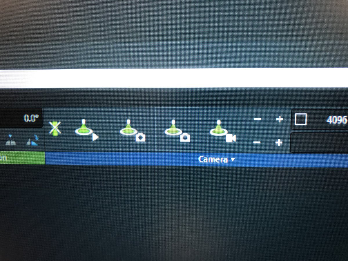
-
Do not change the intensity knob while the screen is lifted. The screen is lifted when
TEMUIshows a black display with dose reading “Unavail”. -
Gold nanoparticles should be visible on screen.
-
-
Explore focus (optional)
-
Press the
z-axisbuttons to observe how focus affects the image.Underfocus — edges appear bright with white Fresnel fringes:
On focus — minimal fringe contrast:
Overfocus — contrast inverts, dark fringes at edges:
-
2.2 C1A1 correction
C1A1 corrects first-order aberrations in the image-forming lenses: defocus (C1) and 2-fold astigmatism (A1).
-
Set underfocus
-
Press
Z-axisdown until you see 4-5 rings in the FFT (slight underfocus). The rings indicate Thon rings from the amorphous carbon, which the corrector software uses for aberration measurement.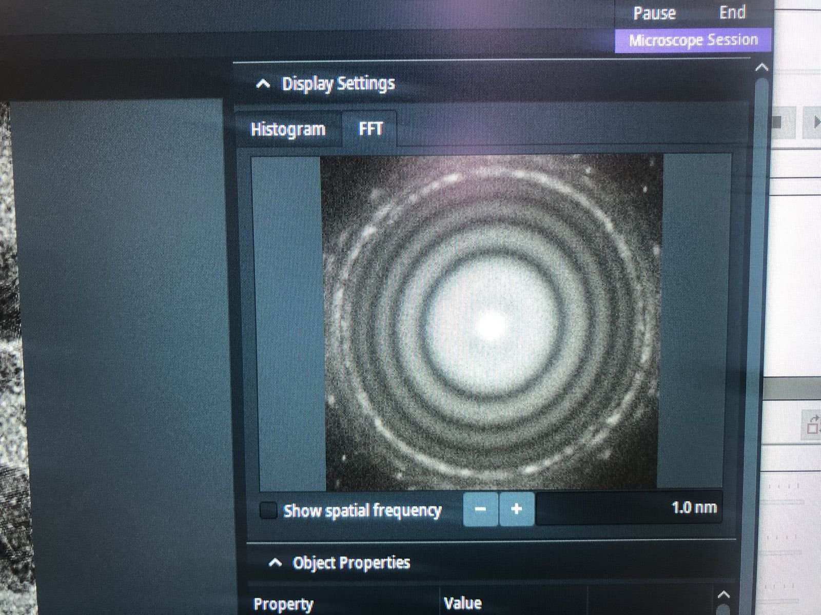
-
-
Reset stigmator values
-
Stop live scanning by clicking the play button in
Velox. -
In
TEMUI, go to theStigmatorquick tab. ResetObjectiveandImage A1to zero. If non-zero, right-click each button to reset, then clickDone.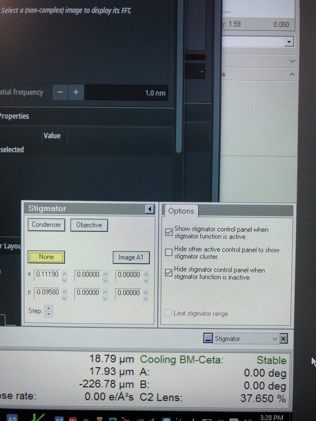
-
-
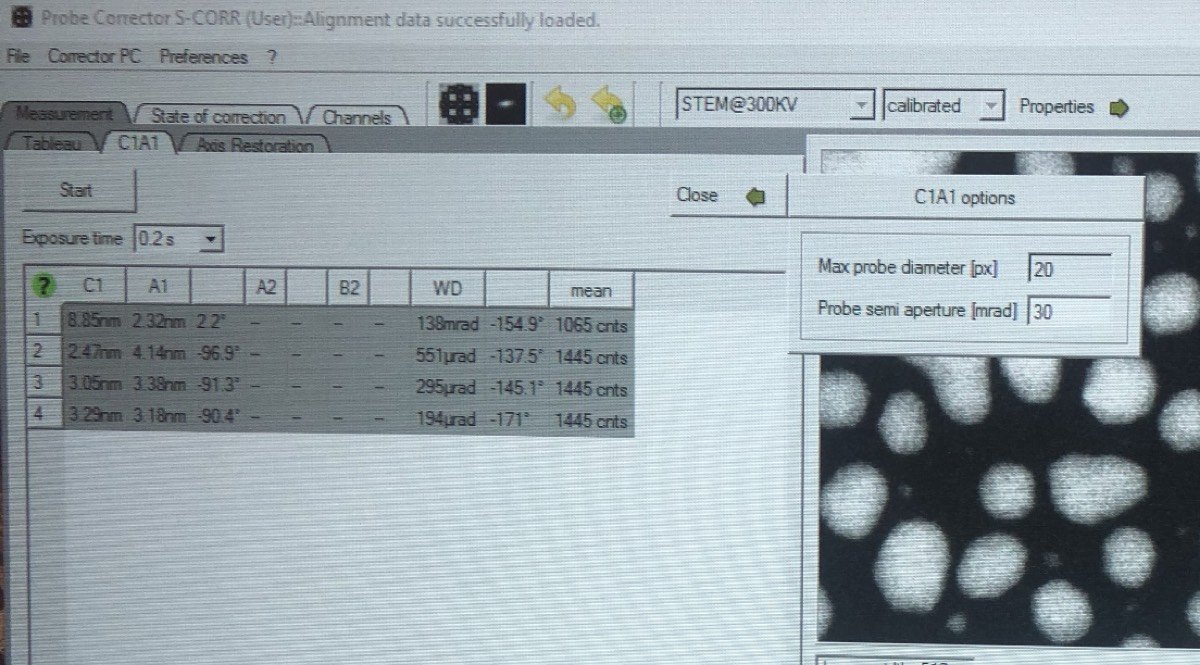
Run C1A1
-
Open the
ImageCorrectorsoftware (top left monitor). -
Set exposure time to 0.3s.
-
Go to the
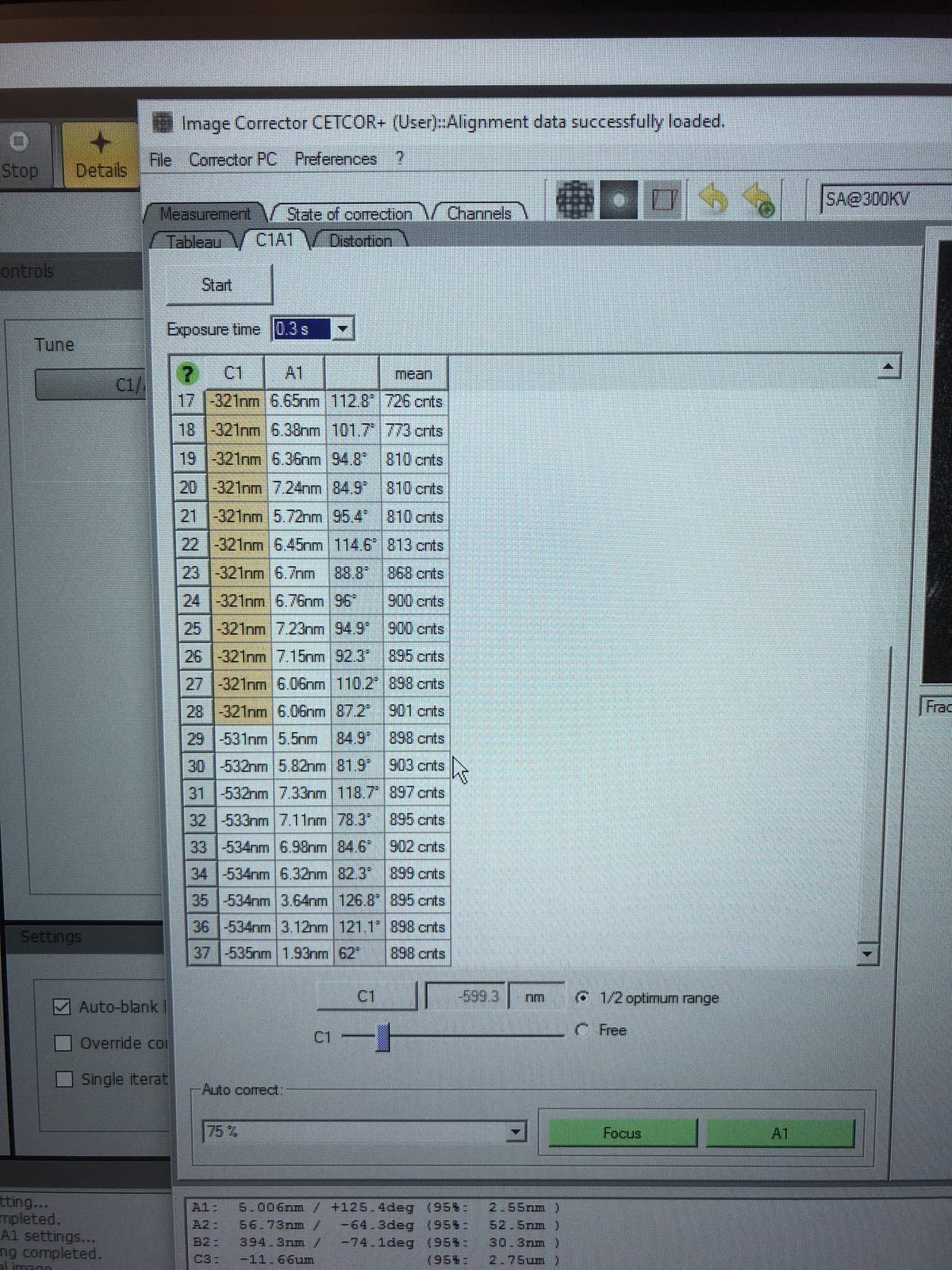
C1A1tab and clickStart. The microscope wobbles the focus up and down (changing objective lens current). The FFT is captured and its ring symmetry, angular distribution, and ring spacing are analyzed. -
During the iteration, carefully set intensity to 800–900 counts by adjusting the intensity knob so the corrector has enough signal.
-
Under
Auto correct, set to75%, then pressFocusandA1during the iteration to apply corrections. -
Aim for
A1< 5 nm. IfC1shows orange, manually adjust the Z-axis during the iteration.C1should be close to the suggested value (in the image above, the software suggests C1 of −599.3 nm).
-
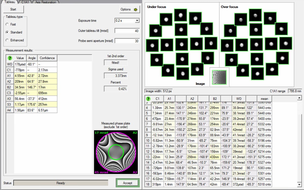
2.3 Tableau measurement
Tableau measures higher-order aberrations by acquiring images at multiple beam tilts. This is necessary for sub-angstrom resolution.
-
Run Tableau
-
In
ImageCorrector, go to theTableautab, selectStandardnext toTableau type, then clickStart.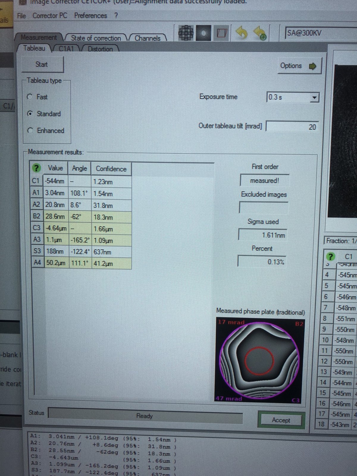
-
-
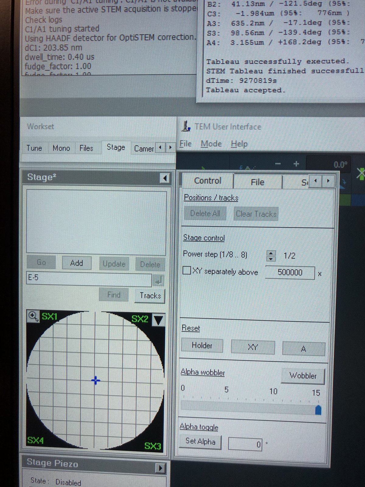
Verify results
-
After the iteration completes, verify the aberration values match the targets below, then click
Accept:Parameter Resolution < 0.10 nm (20 mrad) Resolution < 0.08 nm (24 mrad) A1 < 5 nm < 5 nm A2 < 100 nm < 50 nm B2 < 100 nm < 50 nm C3 ~ −8 μm ~ −8 μm A3 < 5 μm < 1.5 μm S3 < 5 μm < 1 μm -
In
Velox, click the camera button to capture an image and verify improvements.
-
2.4 Save optics settings
-
Save register
-
In
TEMUI, go toFiles, thenSBL FEG Registers. -
Add name
300KV-TEM-<NAME>and clickAdd.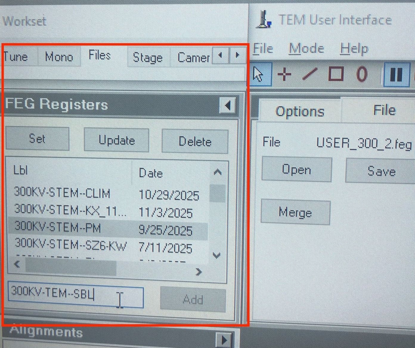
-
-
Verify corrected image
- In
Velox, click thePlaybutton to start live imaging and verify the aberration-corrected image quality. - Done. You are now ready for STEM probe alignment.
- In
Appendix
Reference images (click to expand)
Gray colors during C1A1 probe correction:
Seeing gray colors like below?
In Velox, click Auto-tune. Increase the signal until it touches the red and blue dotted lines:
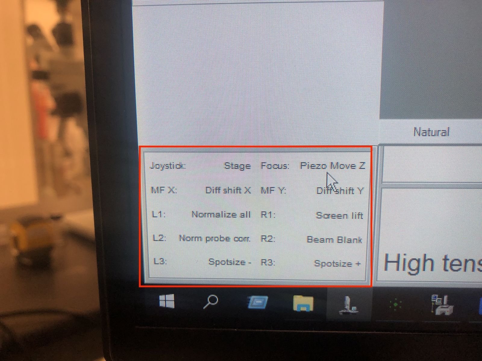
Hand panel R1, R2, R3 values:
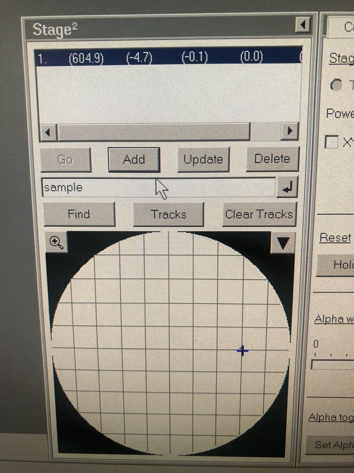
Stage position and coordinates:
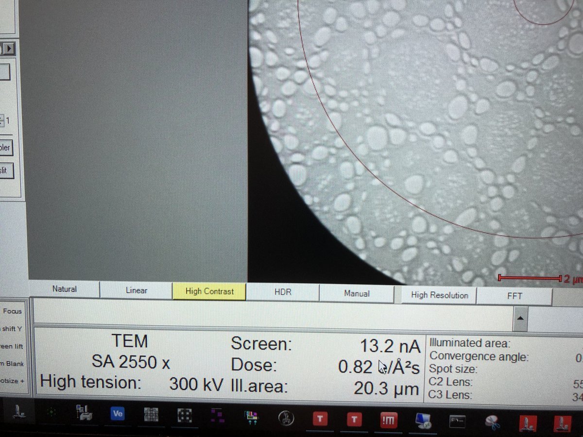
Dose rate and TEM mode display:
HAADF detector on TEMUI:
Samples with holes:
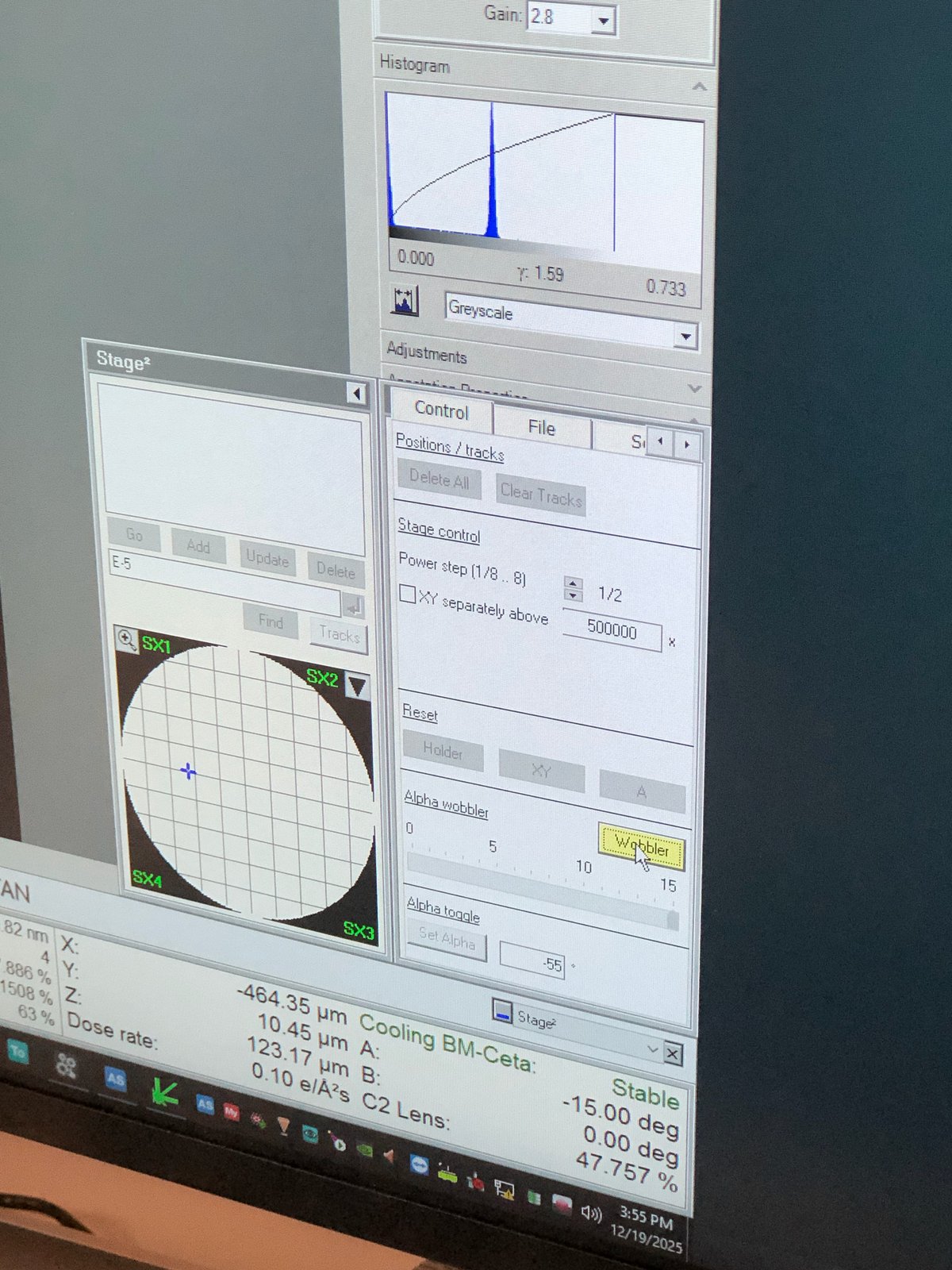
Wobbler to check eucentric height:
At eucentric height, tilting the holder should induce minimal shift.
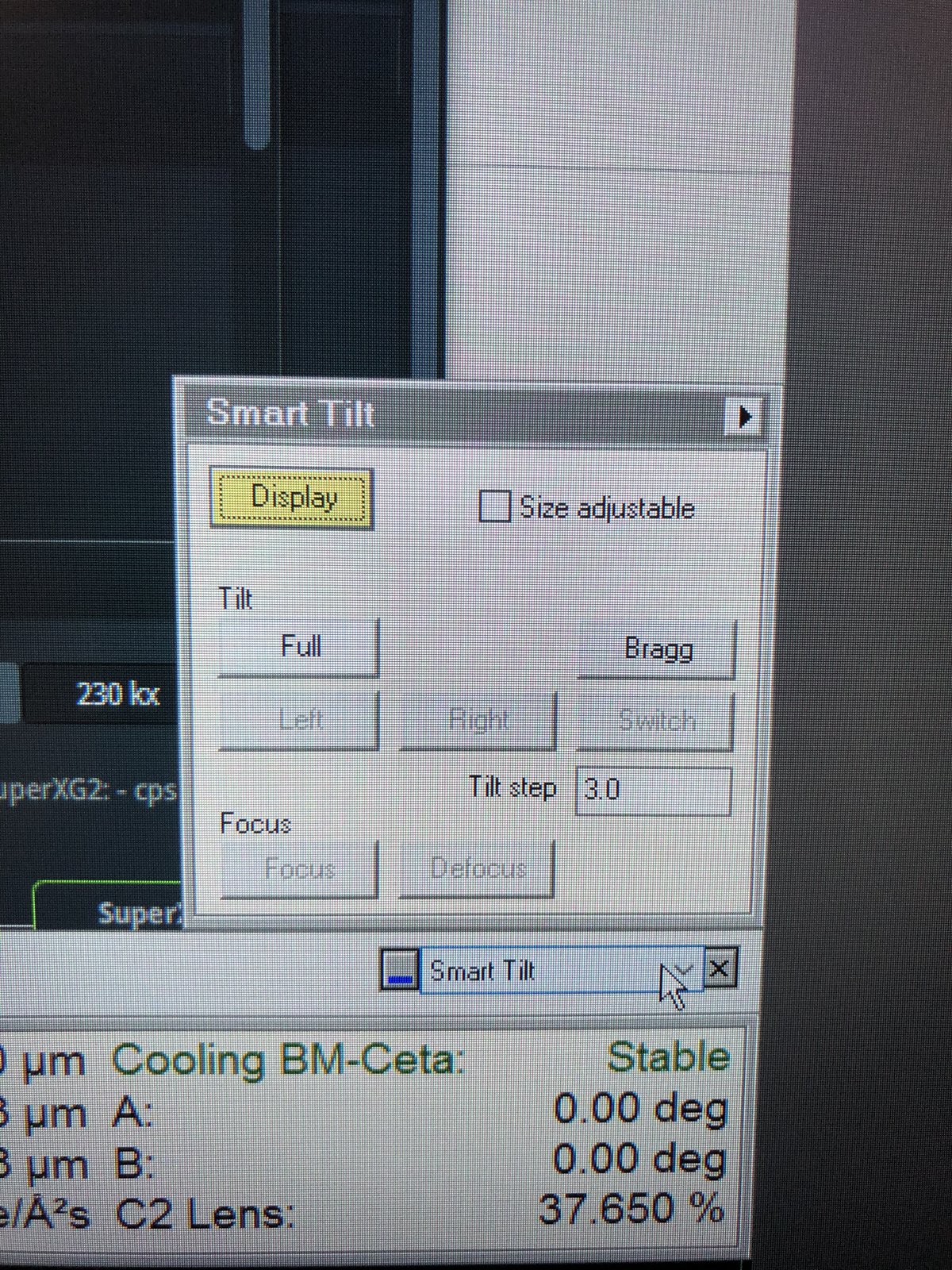
Smart tilt:
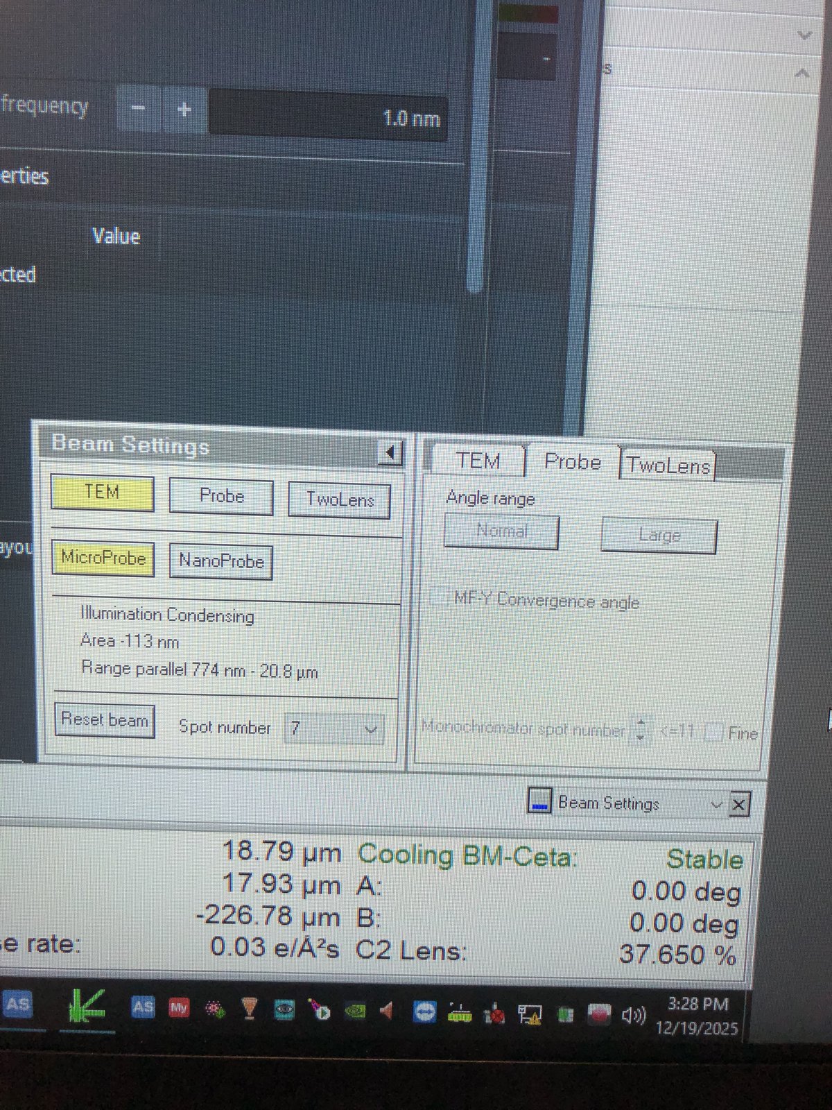
Beam setting in Quick tab:
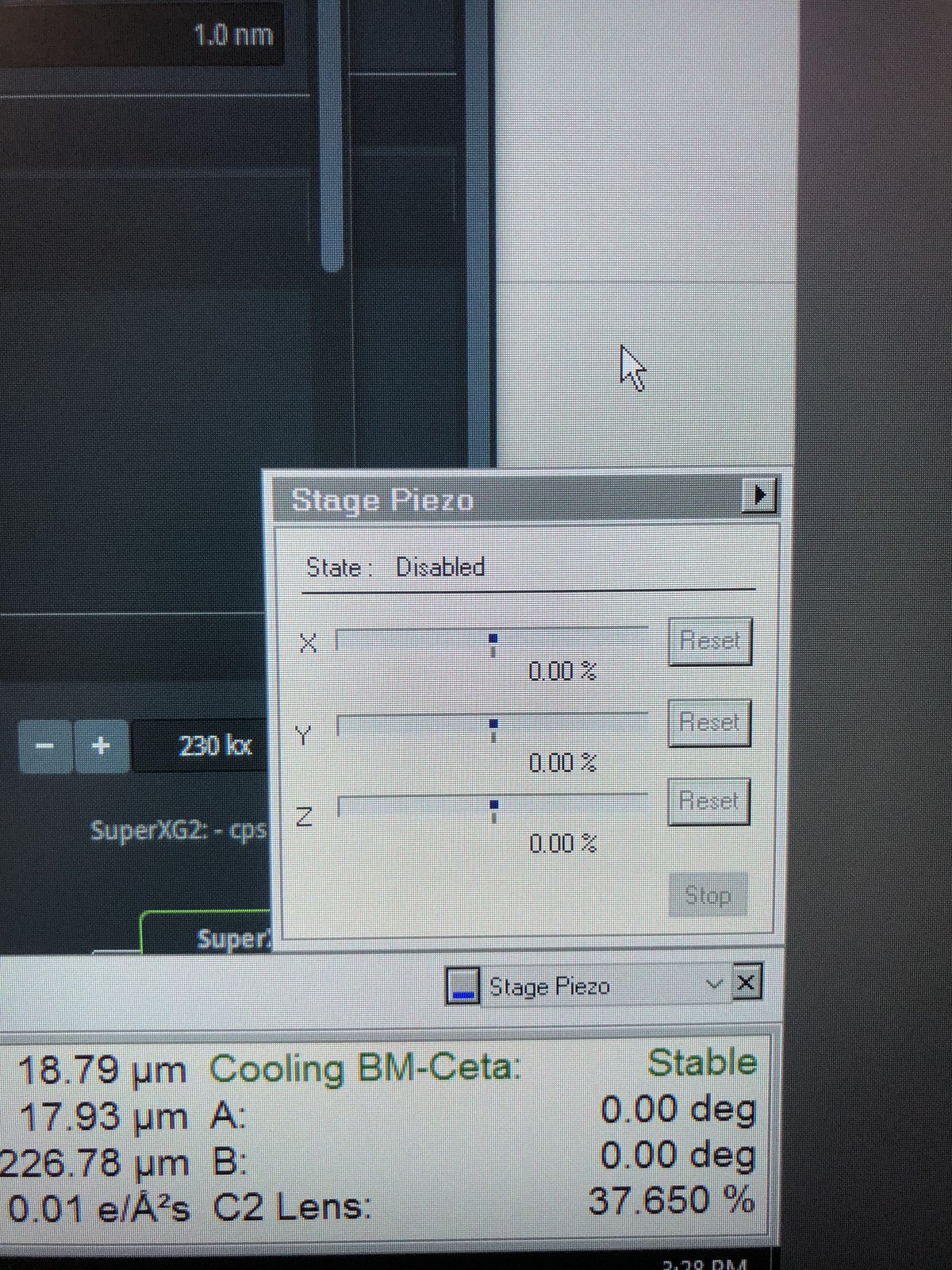
Stage piezo in Quick tab:
Stage tab:
Troubleshooting
Common problems encountered during TEM sessions.
| Problem | Cause | Solution |
|---|---|---|
| Beam is not round after C2 alignment | Condenser astigmatism | Go to Stigmator, then Condenser, adjust mulXY knobs |
| Beam shifts when changing magnification | Beam Shift not set | Use Direct Alignment, then Beam Shift to store center position |
| Image drifts when tilting | Eucentric height not set | Re-do eucentric height (1.3) |
| C1A1 shows orange for C1 | Focus too far from target | Manually adjust Z-axis during iteration |
| Tableau values outside specification | Higher-order aberrations uncorrected | Run additional Tableau iterations, reduce Auto correct to 75% |
| Gray image in Velox during C1A1 | Intensity too low for corrector | Adjust intensity knob to 800-900 counts during iteration |
| No beam visible after opening column valves | Beam is blanked or screen not inserted | Check beam blank status, verify screen position |
FAQ
Convergence angle: In TEMUI, go to Beam Setting, then Probe, and use the mulXY knobs to adjust.
Tableau and C1A1: Tableau measures aberrations visually across multiple tilt angles. C1A1 corrects first-order aberrations (defocus and astigmatism). Run C1A1 first, then Tableau for higher-order corrections.
Underfocus direction: Counterclockwise on hand panel, Z-axis down.
Eucentric height: The z-position where tilting does not shift the sample. At eucentric height, defocus = 0 and probe size is smallest relative to the sample.
Beam Shift vs hand panel ball: Beam Shift stores the center position internally, so the beam stays centered when changing magnification. The hand panel ball moves the beam but does not save the position.
Underfocus vs overfocus: Underfocus produces bright white Fresnel fringes at edges. Overfocus inverts the contrast with dark fringes.
Monochromator: Filters the electron beam to select a narrow energy range, improving energy resolution for EELS and reducing chromatic aberration.
Two-lens vs three-lens mode: Two-lens mode (C1+C2) turns off C3, providing a simpler beam path for C2 aperture alignment. Three-lens mode (C1+C2+C3) is the standard operating mode for TEM imaging.
Objective lens in TEM: In TEM, the objective lens sits below the sample and forms the first magnified image. In STEM, it sits above the sample and focuses the probe.
C2 aperture purpose: The C2 aperture blocks off-axis electrons, controlling the convergence angle and beam current. It must be centered on the optical axis for symmetric beam expansion.
References
Changelog
- Mar 1, 2026 - Restructure to match STEM guide format with subsections, checklists, and troubleshooting table
- Dec 15, 2025 - Add pre-probe corrector with STEM Direct Alignment steps by @bobleesj
- Dec 12, 2025 - Add STEM training images by Guoliang Hu
- Dec 8, 2025 - First draft of Spectra training by @bobleesj
Spectra 300 STEM Alignment Guide (DRAFT)
This guide covers STEM alignment on the Spectra 300 at Stanford SNSF (Stanford Nano Shared Facilities). Screenshots and instructions are provided by Andrew Barnum. Written instructions and images are organized by Sangjoon Bob Lee.
Check before starting your session
First, visually confirm the following from the previous user to ensure no damage has occurred.
- Standard gold nanoparticle sample on a single-tilt holder is loaded.
- Logbook is checked for any notes from the previous user.
- Start your session on NEMO.
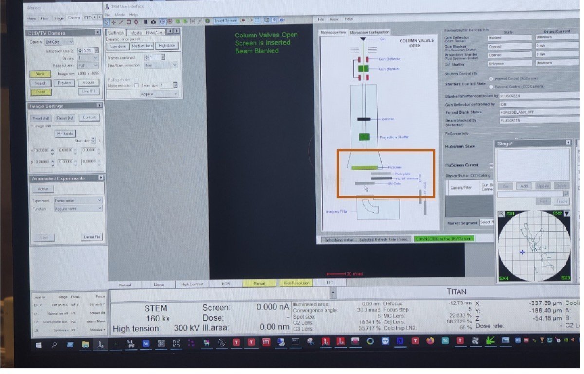
- Screen is inserted.
- Beam is blanked.
- Column valves are closed.
- Turbo pump is off.
- Stage tilt is at 0° (alpha and beta) and the stage has been reset.
- Arina detector is retracted.
- Arina detector is turned off.
- All holders are capped and placed in the holder box.
- No errors are found across all software programs including TEMUI.
Report immediately in the logbook if anything has occurred or contact supervisors.
After you have checked the states,
- Follow any special instructions and warnings posted on NEMO.
- Emergency contacts are available.
Acronyms:
mulXY- Multifunction X/Y knobs on hand panelTEMUI- TEM User Interface (software)
Workstation layout:
| Monitor | Software | Purpose |
|---|---|---|
| Bottom left | TEMUI | Microscope control, vacuum, alignments |
| Bottom right | Velox | Live imaging, acquisition |
| Top left | Probe Corrector S-CORR | Aberration measurement & correction |
| Top right | Velox image gallery | Captured images from Velox |
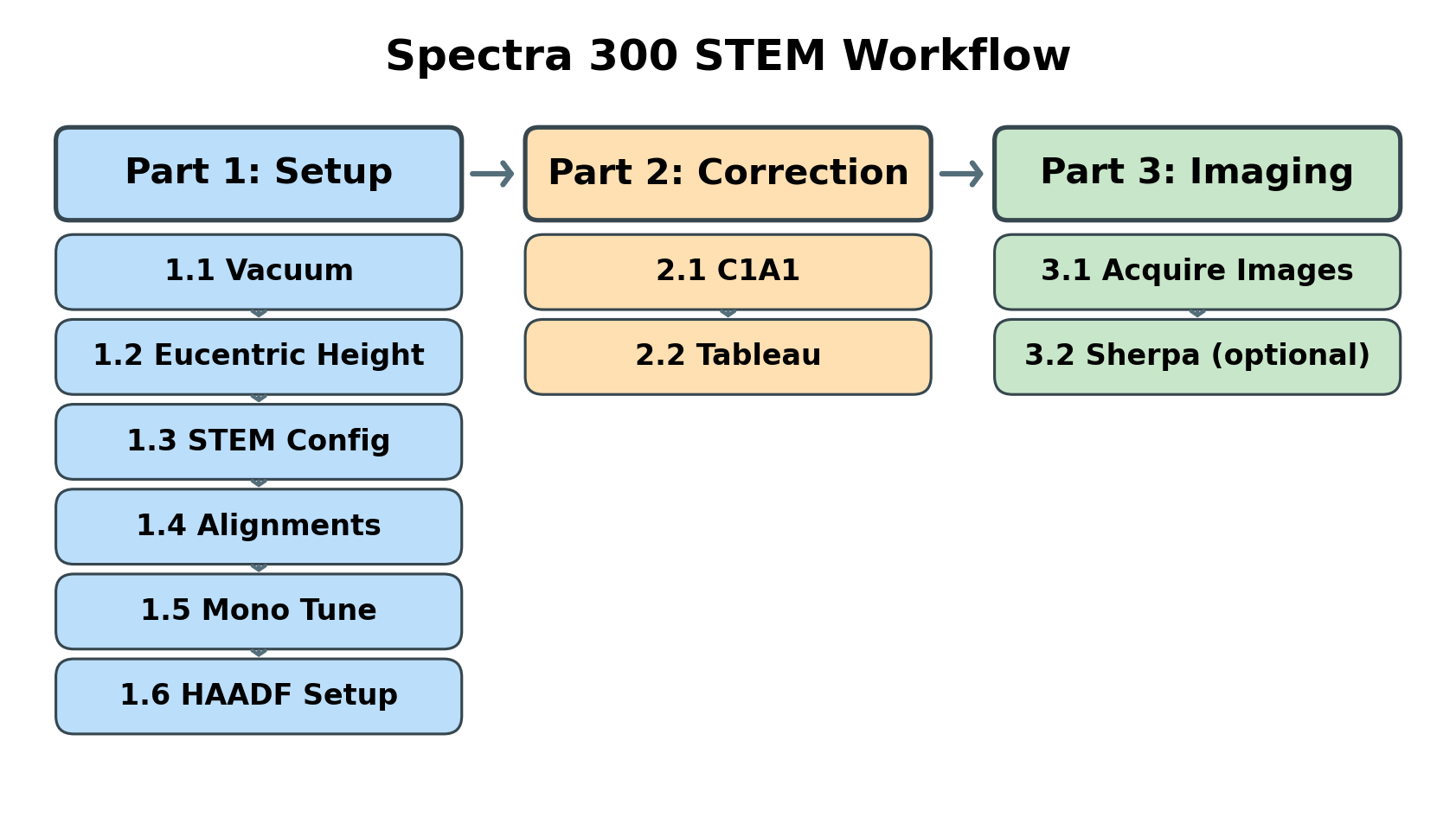
Overview
This guide covers three main phases:
| Phase | Procedures | Time |
|---|---|---|
| Part 1: Setup & Alignment | Vacuum check, eucentric height, STEM mode configuration, direct alignments, monochromator tune, HAADF setup | 5-10 min |
| Part 2: Probe Correction | Correct aberrations (C1A1, Tableau) to achieve sub-angstrom probe | 10-15 min |
| Part 3: Imaging | Image acquisition, Sherpa fine-tuning (optional), load your own sample | varies |
| Part 4: End session | Reload standard sample, pre-departure checklist | 5 min |
Part 1: Setup & Alignment
1.1 Vacuum check
Before imaging, verify that the vacuum system is ready and the column valves can be safely opened. Poor vacuum conditions can damage the electron source and contaminate the sample.
-
Check vacuum status
-
In
TEMUI, openSetuptab. -
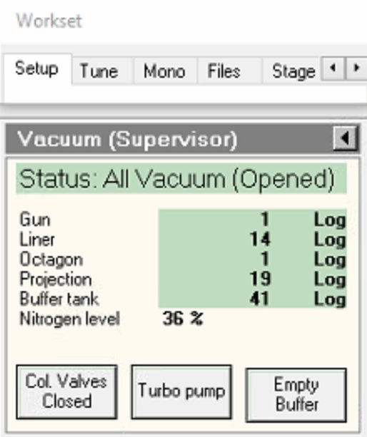
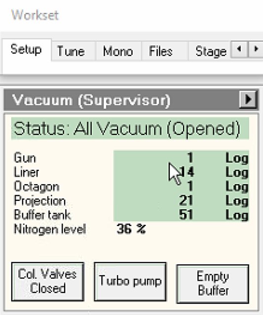
Locate vacuum status panel. Status shows “All Vacuum (Closed)” and
Col. Valves Closedbutton is yellow.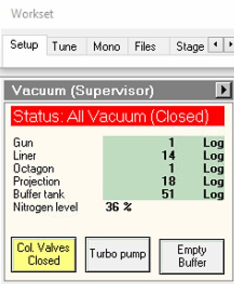
-
-
Verify vacuum pressure
-
Check vacuum pressure values on the log scale (lower = better):
Gauge Typical Log Value Notes Gun 1 Critical for source lifetime Liner 14 Column vacuum Octagon 1 Sample area Projection 19-21 Below sample Buffer tank 41-51 Empty if above 51 -
If buffer tank pressure is above 51, click
Empty Buffer.- Pumps cycle audibly.
-
Wait for value to decrease before proceeding.
-
-
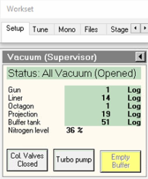
Open column valves
-
Click
Col Valves Closedbutton.- Status changes to “All Vacuum (Opened)”.
NOTE: The system only allows opening if vacuum levels are acceptable. Once opened, the electron beam path is clear from gun to sample.
-
1.2 Check convergence angle
For this guide, we use a convergence angle of 30.0 mrad.
- In
TEMUI, navigate to theTunetab, then selectAperture. - Set Condenser 1, Condenser 2, and Condenser 3 to
2000,70, and1000.
NOTE: These aperture values determine the convergence angle. For example, setting Condenser 2 to
50instead of70gives a convergence angle of 21.5 mrad. A smaller aperture restricts the beam to a narrower range of incident angles, blocking higher-angle electrons.
1.3 Find eucentric height
Complete eucentric height alignment after loading each sample and before imaging. Do not skip this step. At eucentric height, the sample remains stationary when tilted. This is essential for accurate imaging and tomography. The ronchigram “blow-up” method provides a quick way to find this position.
-
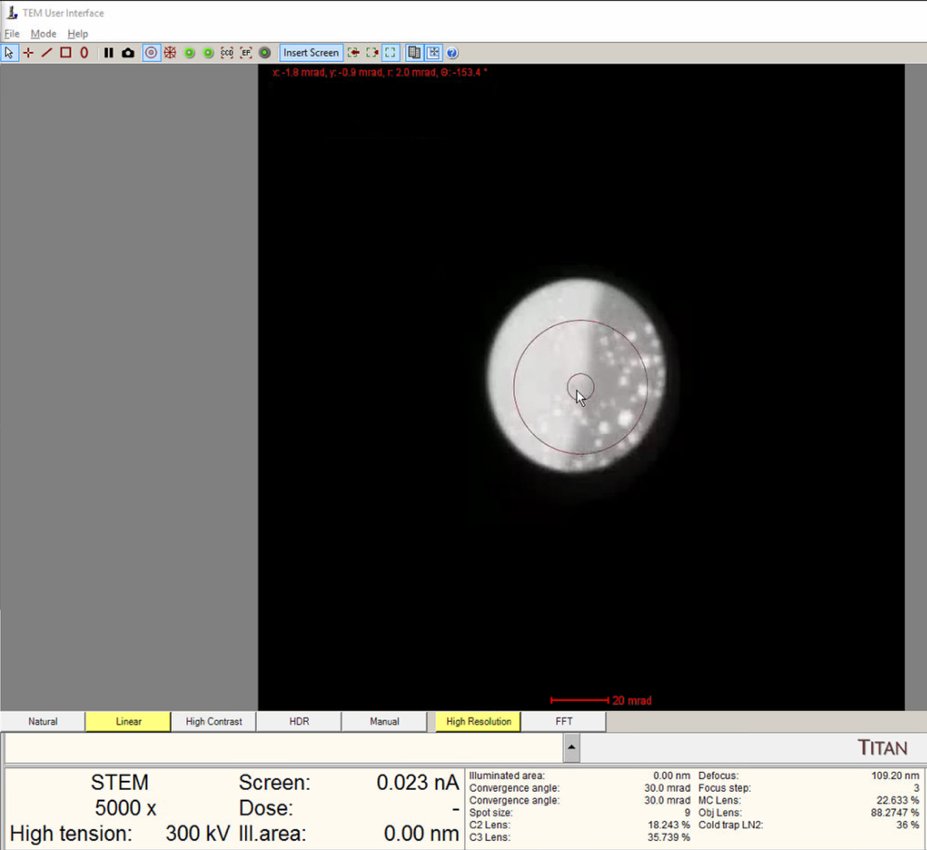
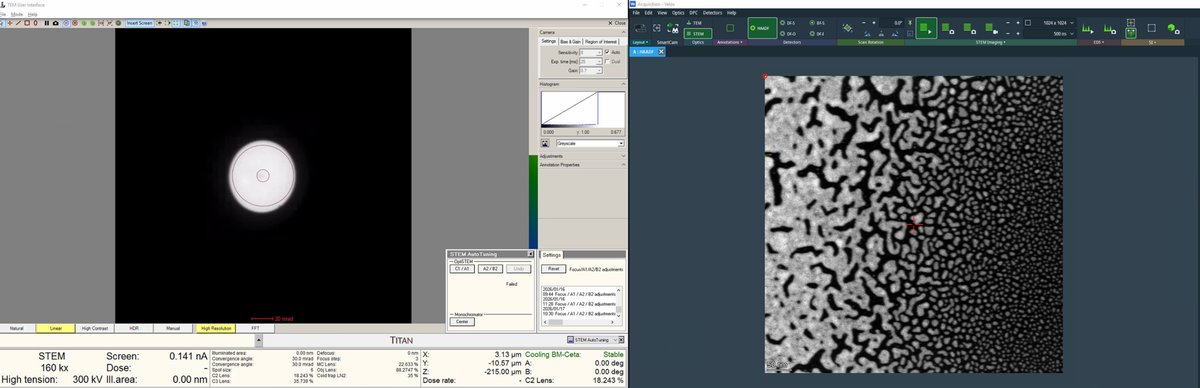
View ronchigram
-
Verify the
Diffractionbutton is pressed on the hand panel with the red light turned on.NOTE: The ronchigram is the diffraction pattern formed when the convergent probe is stationary. When defocused, it contains shadow images of sample features, making structure visible during z-height adjustment.
-
In
TEMUI, view the ronchigram in the main display.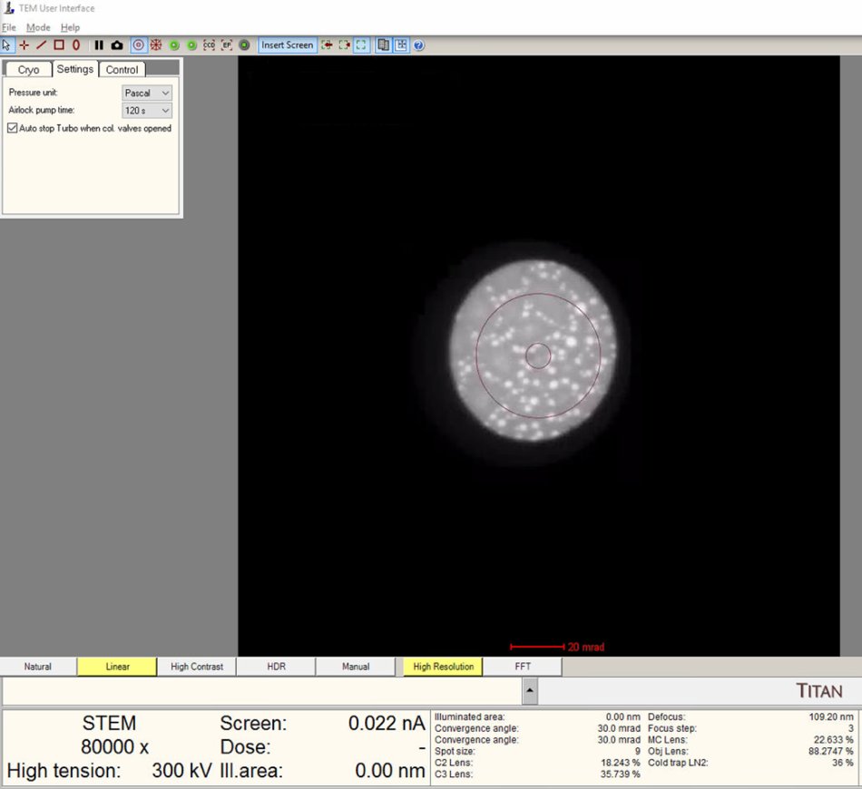
-
Position probe on a sample region that scatters electrons (not over a hole or vacuum).
-
-
Adjust z-axis to find blow-up point
-
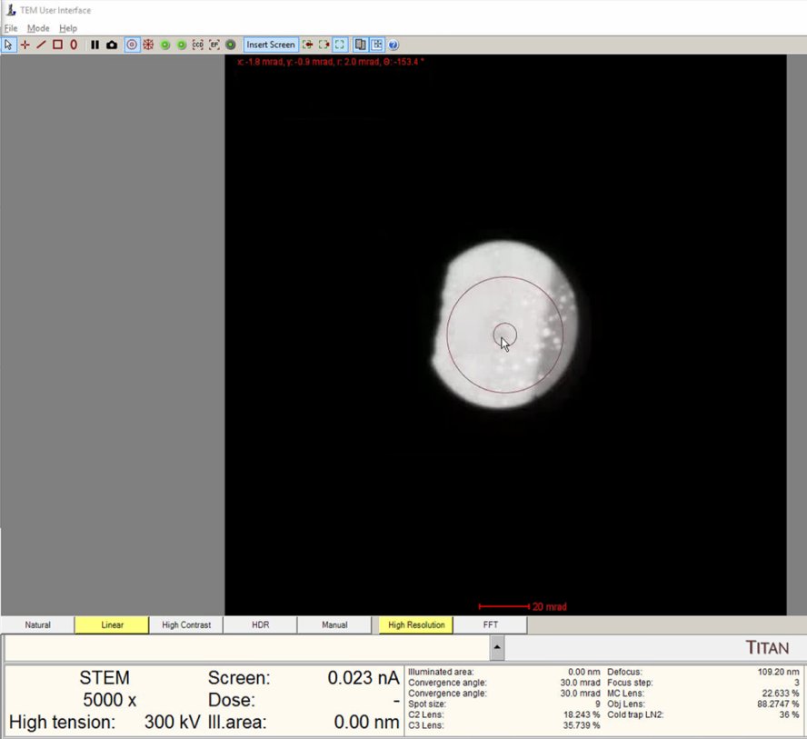
Lower magnification to 5,000x. A wider field of view makes ronchigram changes easier to observe.
-
Find a region where there is a sharp contrast at a boundary, as shown in the following image.
-
Use z-axis buttons on hand panel to move stage up or down.
- Buttons are pressure sensitive: press harder for faster movement.
- Start with gentle presses for fine control.
- Notice that as you adjust the z-axis, the ROI also shifts. Use the joystick to remain on the sharp contrast boundary region.
-
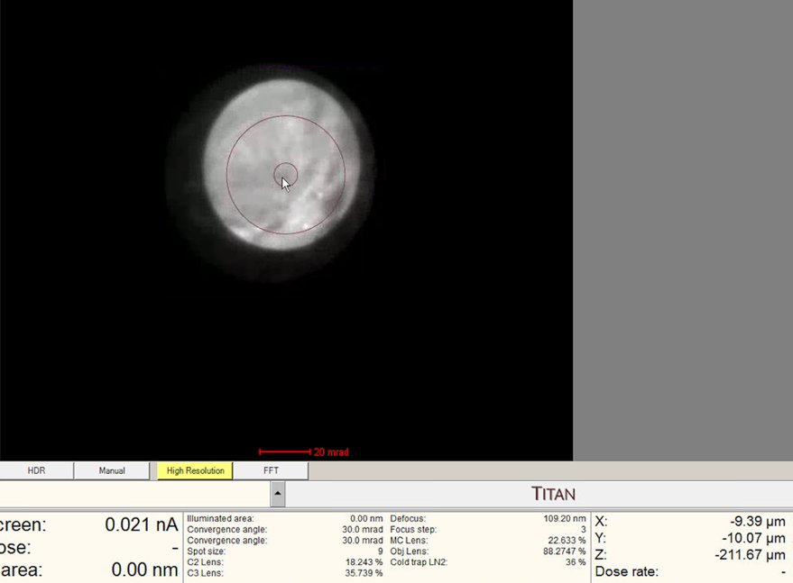
Watch the ronchigram while adjusting z-height. The pattern “zooms” in or out as the sample moves through focus.
-
Continue adjusting. The ronchigram expands when approaching eucentric height, also referred to as the “blow-up” point.
-
Find the “blow-up” point where the ronchigram appears infinitely magnified: shadow image features expand until they fill the entire display.
- If the ronchigram starts shrinking again, reverse direction.
-
1.4 STEM mode configuration
Before performing alignments, configure the STEM imaging parameters and verify detector settings.
-
Enable descan
-
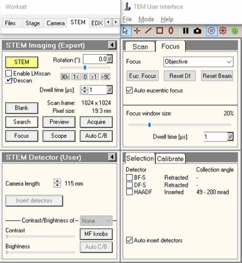
In
TEMUI, locate theSTEM Imaging (Expert)panel. -
Enable
Descancheckbox.NOTE: Descan compensates for beam movement during scanning, keeping the diffraction pattern stationary on the detector.
-
-
Verify HAADF is retracted
-
Locate the
Selectionpanel. -
Verify detector states:
- BF-S (Bright Field): Retracted
- DF-S (Dark Field): Retracted
- HAADF: Retracted
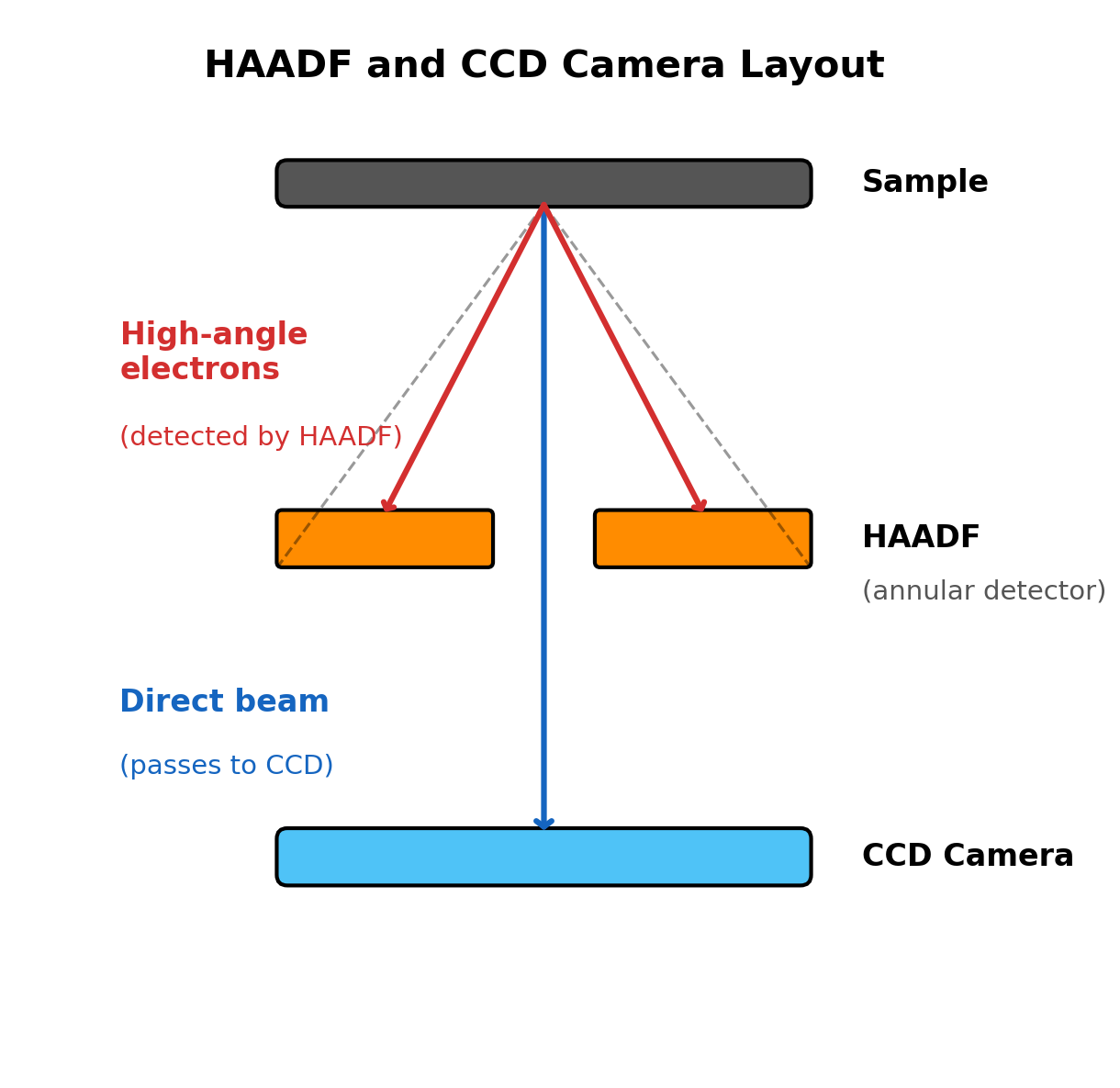
-
Toggle
HAADFcheckbox on then off to confirm retracted state.NOTE: HAADF must be retracted during ronchigram alignment. The HAADF is a ring-shaped detector with a central hole. If inserted, high-angle electrons hit the ring instead of the camera below, blocking part of the ronchigram.
-
-
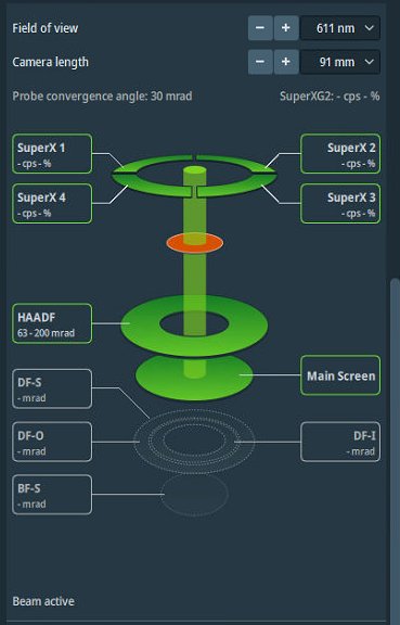
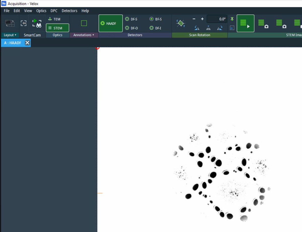
Set detector layout in Velox
-
Open
Veloxacquisition software. -
Open detector layout display.
-
Set camera length to 91 mm.
NOTE: Camera length determines detector collection angles. The layout display shows the angular ranges for each detector.
-
-
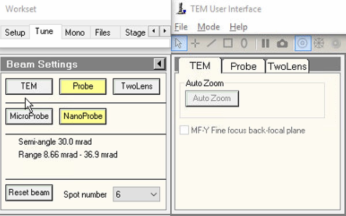
Configure beam settings
-
In
TEMUI, go to theTunetab and locate theBeam Settingspanel. -
Select
Probemode.- Button is highlighted yellow when active.
-
Select
NanoProbemode. -
Set spot number to 6.
NOTE: NanoProbe provides a smaller, more coherent probe than MicroProbe. Lower spot numbers produce smaller probes with lower current; higher numbers produce larger probes with more current.
TODO: Verify spot number convention for Spectra 300. On some Thermo Fisher systems, it is the opposite (spot 1 = most current).
-
1.5 Direct alignments
The basic alignments center the electron beam and align it through the optical column. Proper alignment is essential for optimal resolution and probe symmetry.
-
Set magnification and open Direct Alignments
-
Set magnification to 200-300kX using the magnification knob.
-
In
TEMUI, navigate toTunetab, thenDirect Alignments. This panel provides access to all fundamental beam alignment procedures. -
Select
Diffraction Shift and Focus alignmentto begin.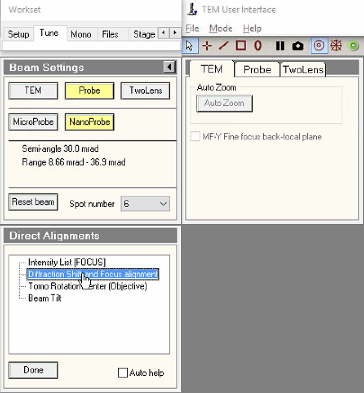
-
-
Center ronchigram
-
Observe the ronchigram position on the display. If the ronchigram is shifted from center, use the
mulXYknobs to bring it back.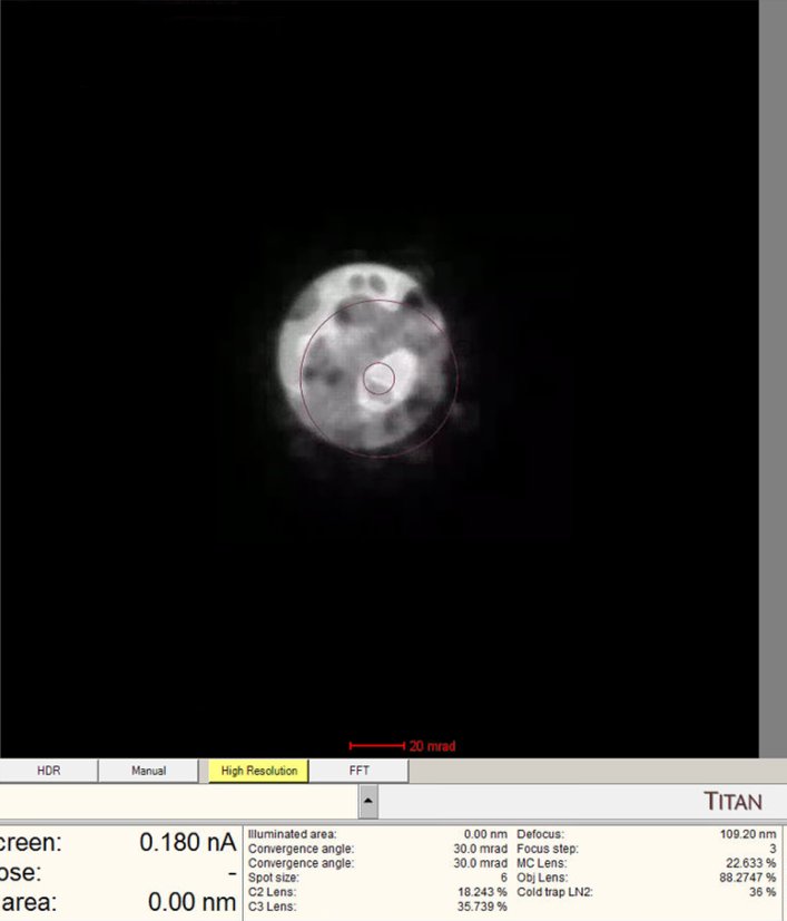
-
The
mulXYknobs now control diffraction shift. Adjust until the ronchigram is centered.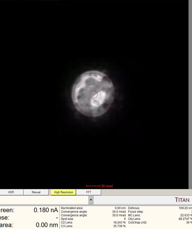
-
-
Reset STEM AutoTuning
-
In the quick dropdown menu, select
STEM AutoTuning. This panel stores automatic alignment adjustments from previous sessions. -
Click
Resetunder Settings to clear stored values. This establishes a known baseline. Previous user adjustments persist and interfere with fresh alignments if not reset.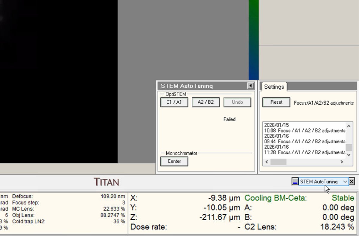
-
-
Switch to probe image mode
-
Press the
Diffractionbutton on the hand panel to enter probe image mode (STEM scanning). The red light should turn off once pressed.No beam found? In the following step you will click
Beam Shiftand adjust themulXYknobs. Watch the screen current: it changes from 0.000 nA to 0.001 nA, etc. This means you are shifting the beam position near the screen. You will see dim light coming from the edges. Press theFineandCoarsebuttons to adjust the sensitivity of themulXYknobs.Still can’t find the beam at all? Try temporarily increasing the C2 aperture from
70to150in theAperturespanel. The larger aperture lets more electrons through, making the beam much easier to locate. Once you find and center the beam, switch back to70before continuing.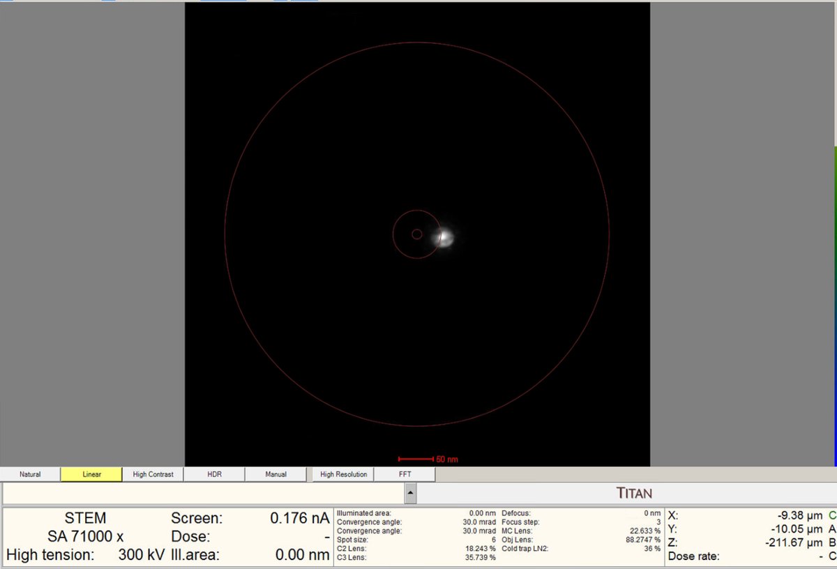
Diffraction mode vs. Probe image mode
Mode Probe Display Diffraction mode Stationary Ronchigram - diffraction pattern from convergent probe Probe image mode Scanning STEM image - probe scans to build up image pixel by pixel The
Diffractionbutton on the hand panel toggles between these two modes.
-
-
Align beam shift
-
Click on
Beam shiftin the Direct Alignments panel. ThemulXYknobs now control alignment beam shift. -
Use the
mulXYknobs to center the beam on the screen. The beam responds smoothly to knob movements. If the beam moves too quickly, pressFineon the hand panel to reduce sensitivity. -
Important: If the beam is lost after clicking beam shift, reduce magnification until the beam is visible, center using the
mulXYknobs. -
Click
Doneonce the beam is properly centered.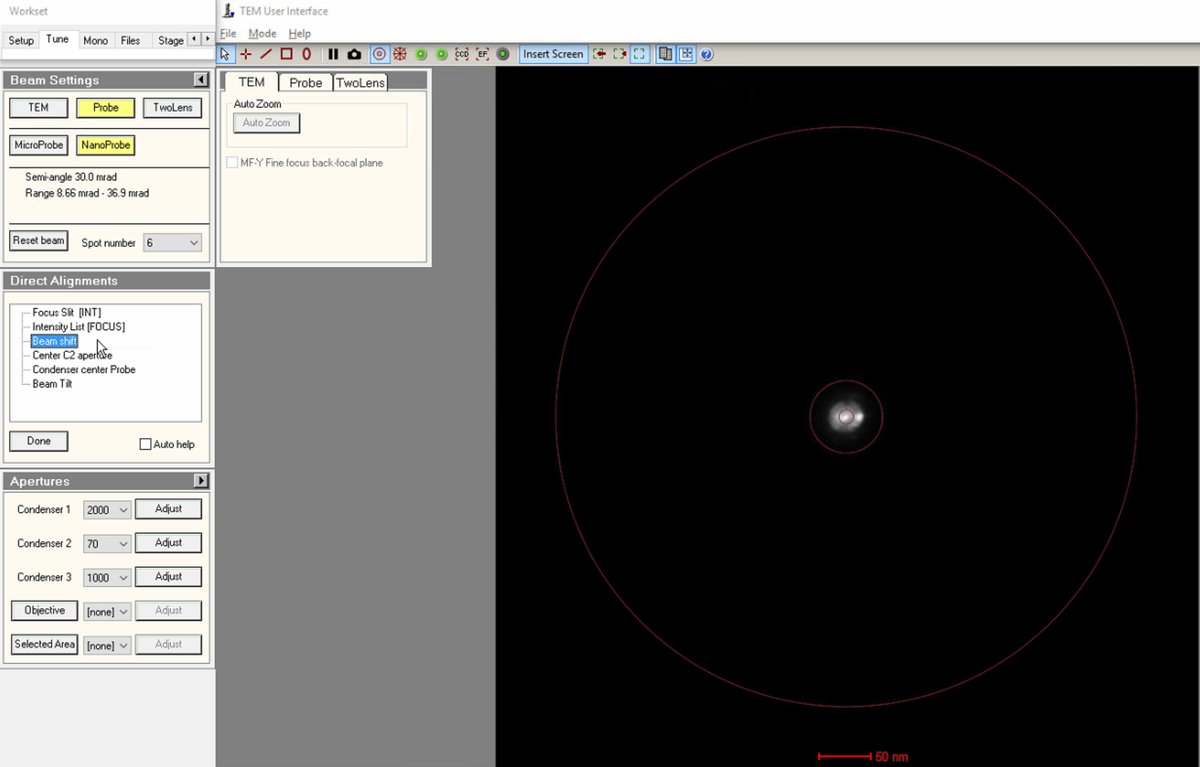
-
-
Center C2 aperture
-
Select
Center C2 aperturefrom the alignment options. The system oscillates the C2 lens, causing the beam to expand and contract rhythmically. -
Watch the beam movement carefully. The beam pulses in and out. The goal is to make this expansion/contraction perfectly concentric (no lateral movement).
-
Use the
mulXYknobs to adjust the aperture position. -
Click
Donewhen the movement is concentric.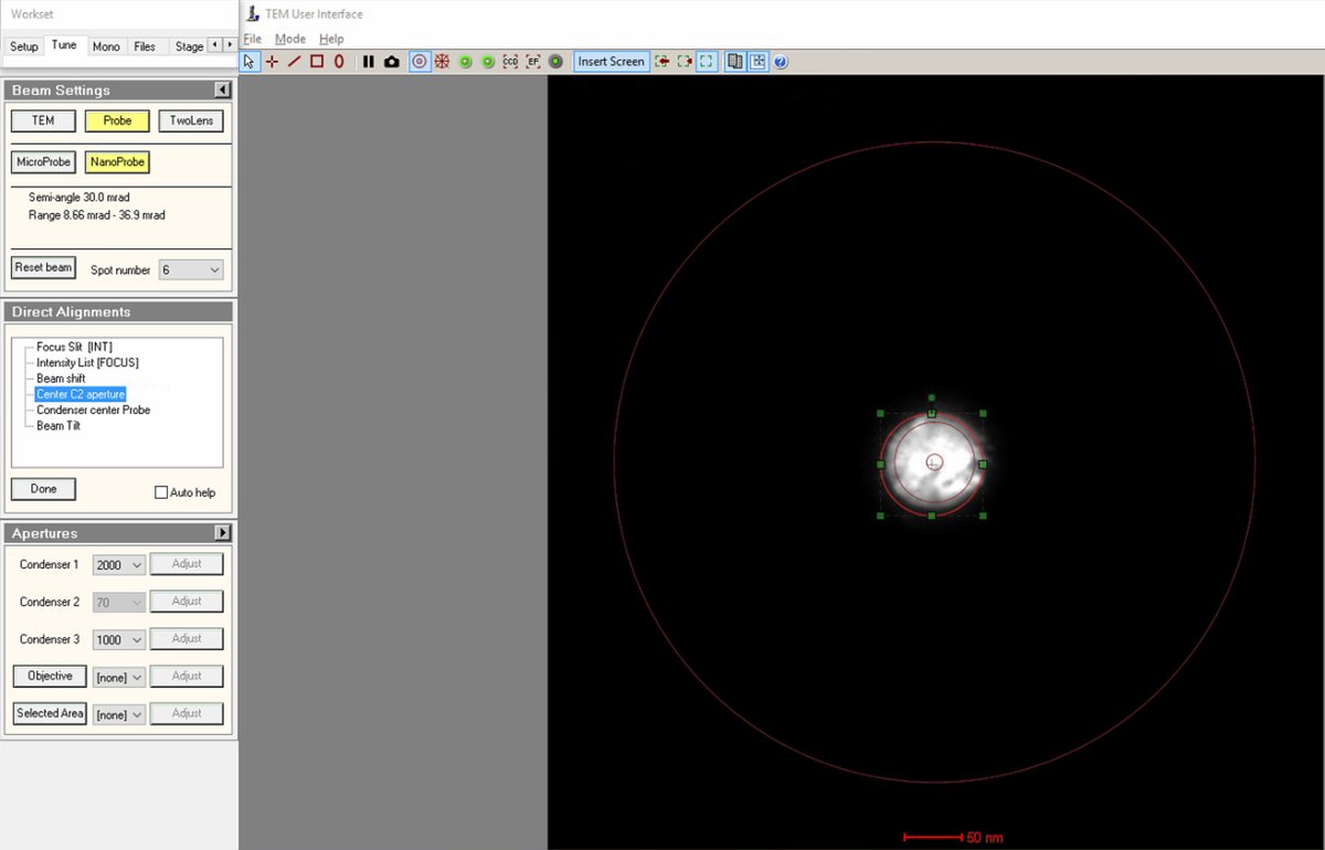
-
-
Align beam tilt
-
Select
Beam Tiltfrom the alignment options. This alignment minimizes the lateral shift of the beam when tilting. -
Use the
mulXYknobs to minimize lateral movement of the beam. When properly aligned, the beam changes angle without shifting position. -
Reduce the lateral x and y movements as much as possible using the
mulXYknobs. -
Click
Doneonce the lateral movement is minimized.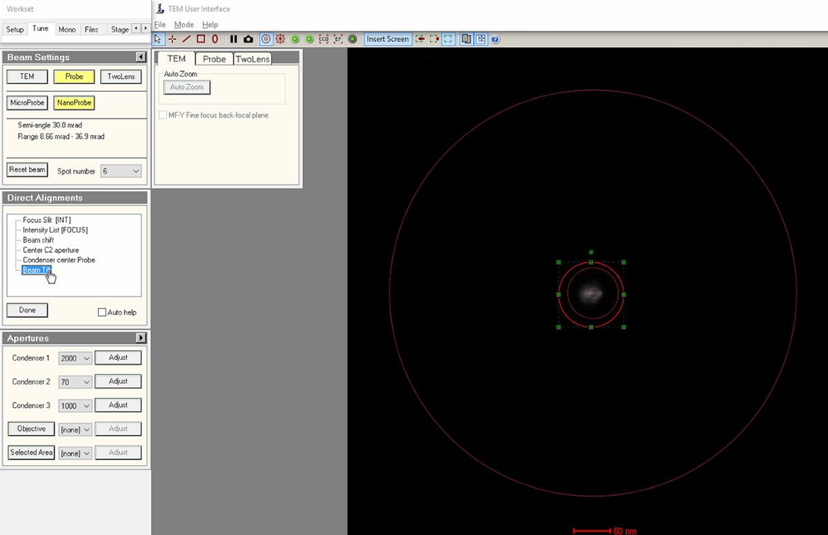
-
-
Verify final diffraction shift
-
Press the
Diffractionbutton on the hand panel to switch back to diffraction mode (view the ronchigram). The red light should now be on. -
Return to
Diffraction Shift and Focus alignmentfor a final centering check. -
Use
mulXYto center the ronchigram precisely on the display. Centering confirms the beam is on the optical axis. -
Click
Doneto complete the direct alignments.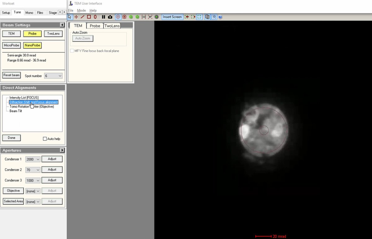
-
Note: Mode changes (diffraction ↔ probe image, TEM ↔ STEM) disable descan. Re-enable descan after each mode switch. If the image looks distorted, verify
Descanis enabled inSTEM Imaging (Expert).
1.6 Monochromator tune
Before proceeding to probe correction, check that the monochromator is properly aligned and not partially blocking the beam. The monochromator selects a narrow energy spread from the electron source, improving resolution but reducing beam current.
-
Open Monochromator Tune
-
In
TEMUI, go to theMonotab and locate theMonochromator Tune (Expert)panel. This panel provides controls for adjusting the monochromator position and focus. -
Click on both
ShiftandFocusbuttons to enable adjustment mode. At this point, the intensity knob controls monochromator focus and themulXYknobs control monochromator shift.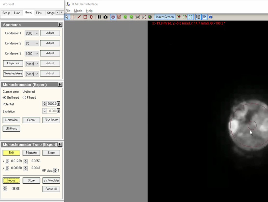
-
-
Adjust focus
-
Adjust the intensity knob to bring the Focus value close to 0. As the monofocus approaches zero, the screen current increases because more electrons pass through the monochromator slit.
-
While adjusting Focus toward 0, also adjust the
mulXYknobs to ensure the beam isn’t blocked. The screen current inTEMUIshould be above 15 nA when focus is near zero.No beam visible? Click
Linearin the detector settings to switch from log to linear display mode. If the beam is still missing, return to the initial focus value and slowly bring it back toward 0 while adjustingmulXY, as in the Beam Shift alignment. -
Watch the current readout while adjusting.
-
-
Center and adjust current
-
Adjust the
mulXYknobs to center the beam through the monochromator.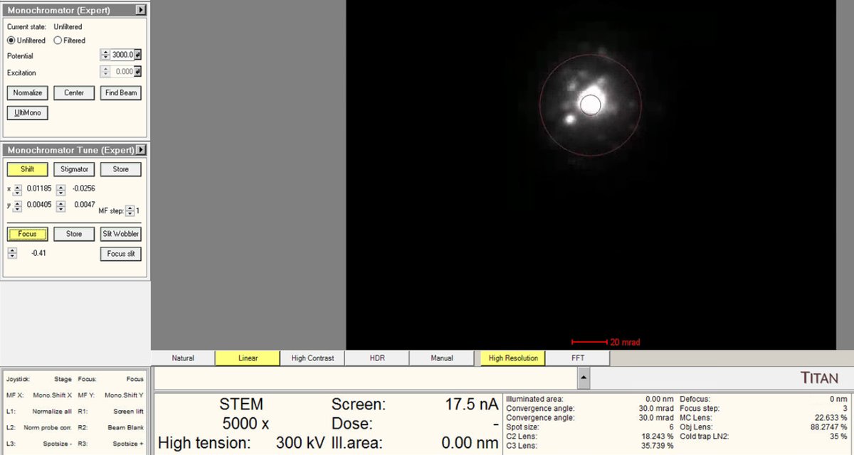
-
Use the intensity knob to achieve the target beam current (~0.150 nA for high-resolution STEM).
-
-
Deselect Shift and Focus
- Click
Shiftagain to deselect both buttons (they toggle together). - This returns the intensity knob and
mulXYknobs to their normal functions. Verify the current readout shows the target value before proceeding.
- Click
-
Re-verify eucentric height
- Use the z-axis controls to return to the “blow-up” point (eucentric height). Monochromator adjustments affect focus; re-verify eucentric height.
1.7 HAADF imaging setup
Before running aberration correction, set up HAADF (High-Angle Annular Dark Field) imaging to view the sample and find a suitable region. HAADF provides Z-contrast imaging where heavier atoms appear brighter.
-
Switch to HAADF
-
In the
Veloxacquisition software, clickSTEMto enter STEM mode, -
Click
HAADF. This automatically inserts the HAADF detector. -
Verify in
TEMUIthat the HAADF detector shows “Inserted” status with the correct collection angle (63-200 mrad).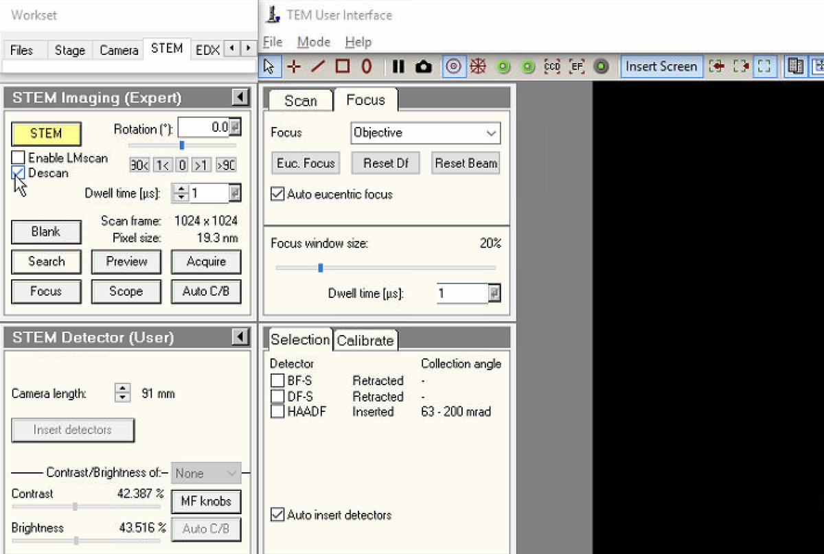
-
-
Verify Descan is enabled
- In
TEMUI, go toSTEM Imaging (Expert)and verifyDescanis enabled. Mode changes disable descan; re-enable after switching modes.
- In
-
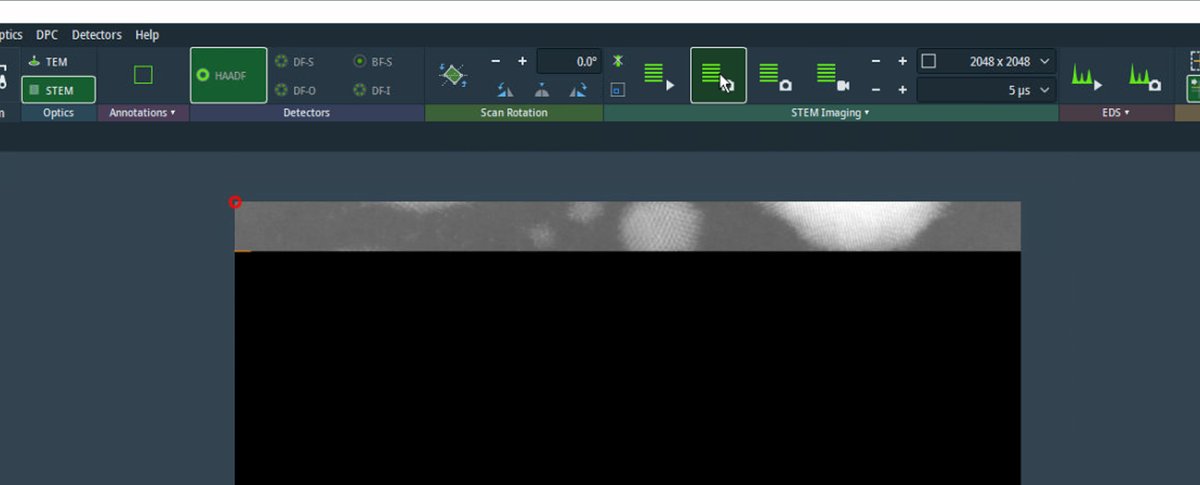
Start live scanning
-
Click the play button in
Veloxto start live scanning. -
The image is saturated (all white) initially. Detector signal adjustment follows in the next step.
-
-
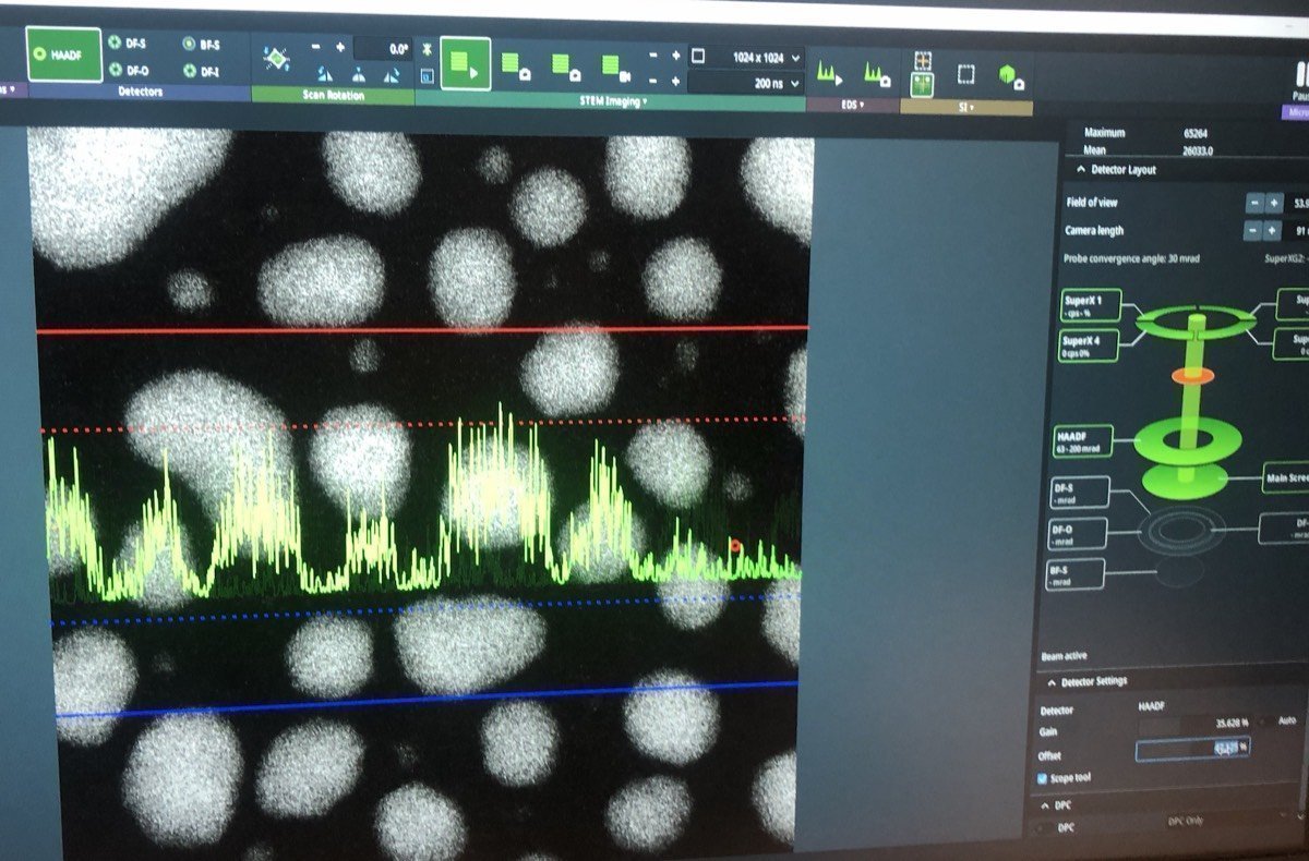
Adjust detector signal
-
In
Velox, clickScope toolto enable signal adjustment. -
Adjust
GainandOffsetso the signal does not go above the dotted red lines.Signal math: Display = (Gain × Signal) + Offset
- Gain (= Contrast): Multiplier that stretches the signal. 100% = no change, 200% = double the contrast
- Offset (= Bias/Brightness): Shifts the baseline as a percentage of the display range
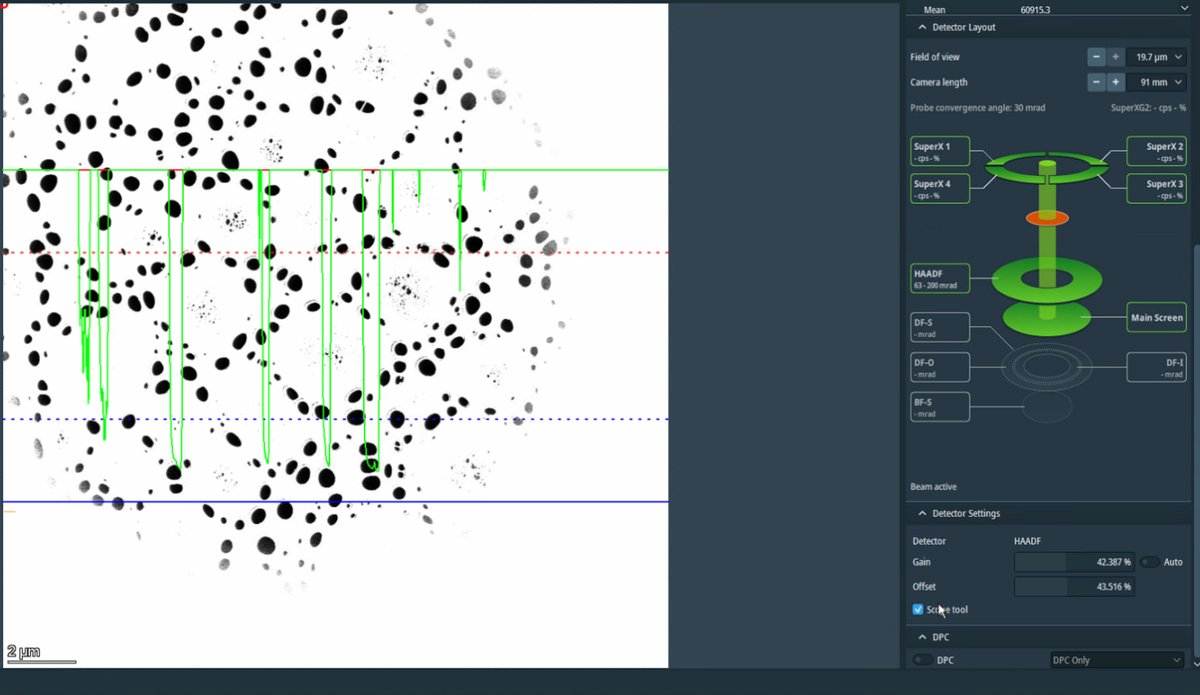
-
If the signal is clipping at zero (bottom of display), increase
Offsetto shift the signal up.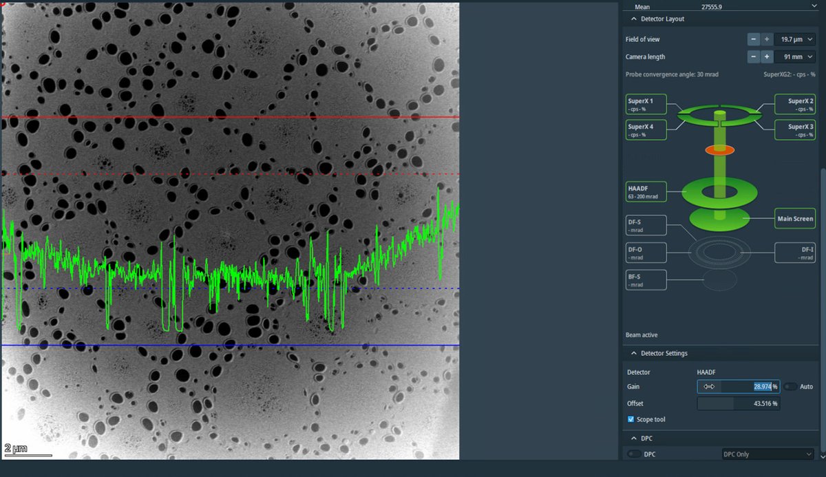
-
Adjust the magnification to ~20,000x using the magnification knob. Once adjusted, uncheck
Scope toolto turn it off.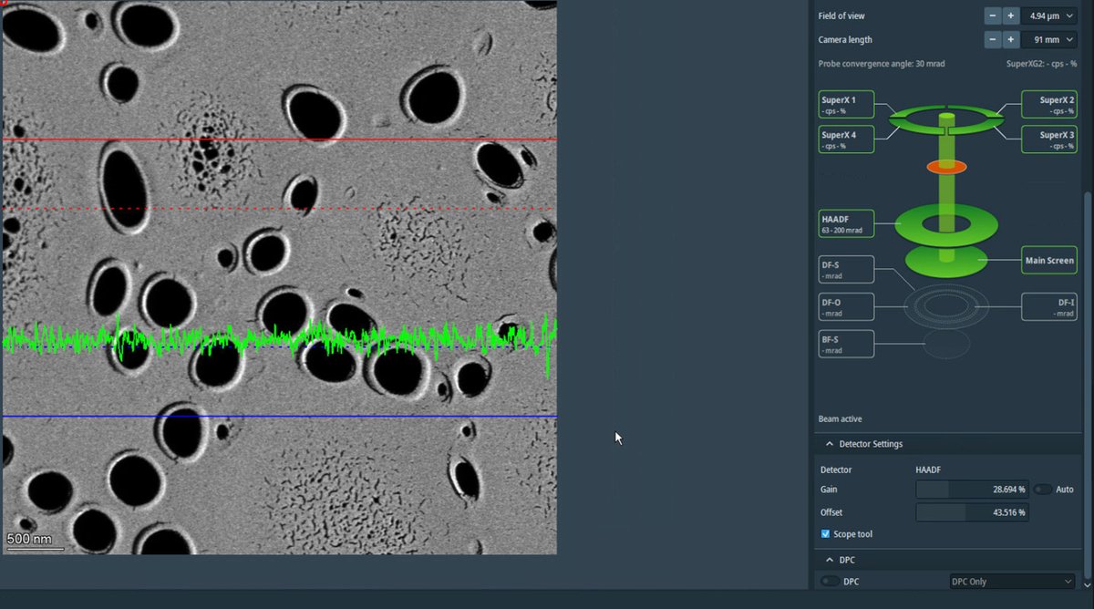
-
-
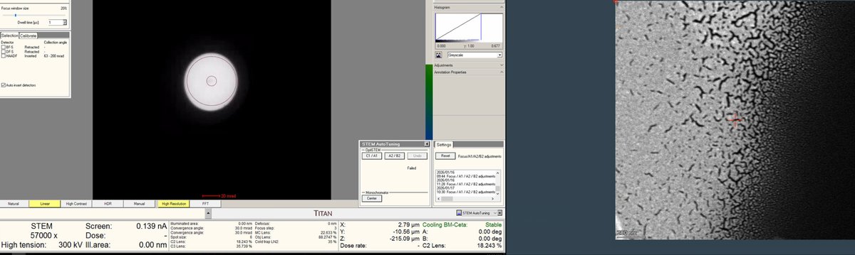
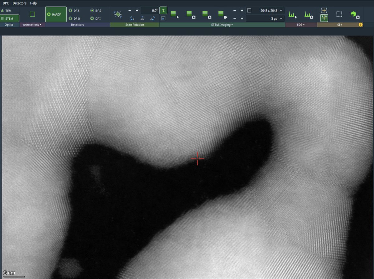
Find sample boundary
-
Reduce magnification to ~10,000x and navigate with the joystick to find a suitable region.
-
Locate a boundary region with particles at the edge of a support film, with vacuum visible.
-
This type of region provides excellent contrast for aberration correction.
-
-
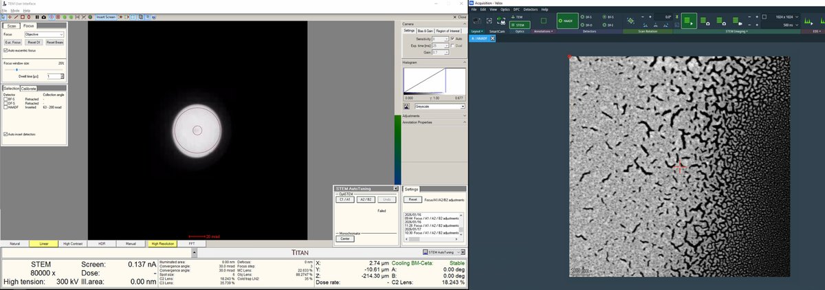
Adjust focus
-
Once a suitable boundary is found, increase magnification to ~160,000x. Alternate between magnification and z-axis adjustments until focus is sharp.
-
Adjust the z-axis while watching the HAADF image. Features become sharper as focus is approached.
-
Continue adjusting magnification and z-axis.
-
Finalize the position with sharp features and distributed particle sizes.
Distributed particles are important for aberration measurement. Aberrations vary with position relative to the optical axis (e.g., coma increases further from center). The correction algorithm requires ronchigram data from multiple positions to accurately fit the aberration coefficients.
-
Part 2: Probe Correction
Before starting probe correction, retract the HAADF detector. C1A1 and Tableau both analyze the ronchigram, and the HAADF ring blocks high-angle electrons from reaching the camera below. In TEMUI, verify the HAADF detector shows “Retracted” status.
TODO: Confirm with staff whether HAADF must be retracted for C1A1/Tableau on Spectra 300 S-CORR.
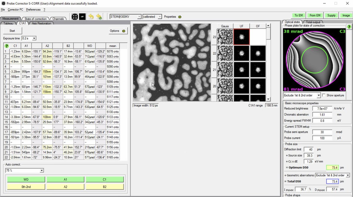
Aberrations distort the electron probe and degrade image resolution. The goal of probe correction is to achieve a flat, aberration-free ronchigram. The figure below shows how individual aberrations affect the ronchigram appearance:
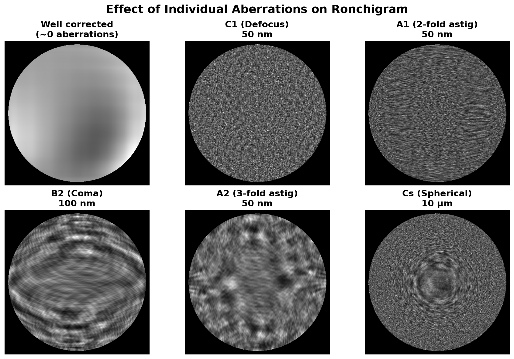
Interactive demo: Explore how aberrations affect the ronchigram at bobleesj.github.io/electron-microscopy-website/ronchigram
Probe correction uses two tools in the Probe Corrector S-CORR software:
| Tool | What it corrects | How it works |
|---|---|---|
| C1A1 | First-order: defocus (C1) and 2-fold astigmatism (A1) | Continuous ronchigram measurement; click buttons to apply |
| Tableau | Higher-order: A2, B2, C3, S3, A3 | Single measurement sequence with beam tilts; then apply |
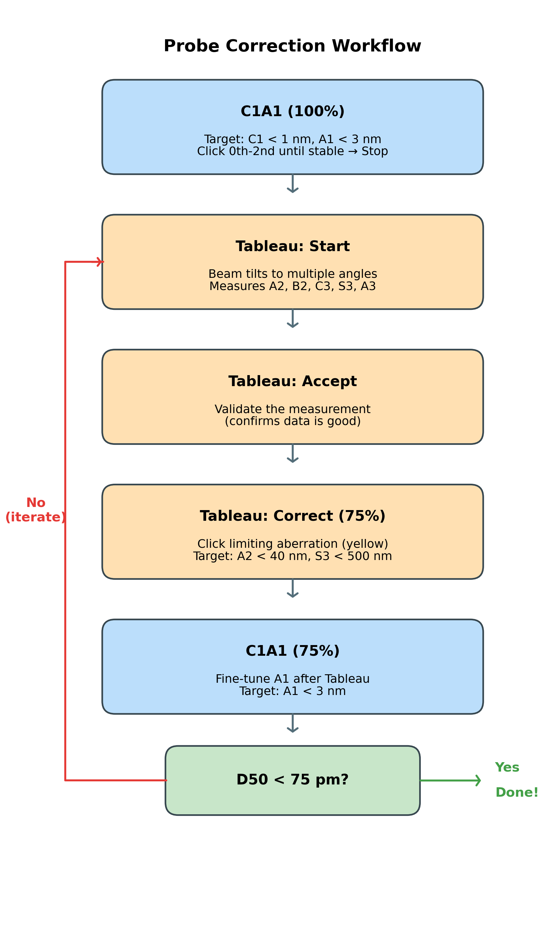
The correction workflow:
The following workflow is covered in this section. Follow the steps below, then use this diagram as a quick reference:
2.1 C1A1 correction
C1A1 corrects first-order aberrations: defocus (C1) and 2-fold astigmatism (A1). These are the dominant aberrations that must be corrected before higher-order Tableau measurement. The C1A1 procedure analyzes the ronchigram to measure and correct these aberrations iteratively.
-
Open Probe Corrector
-
On the top left monitor, open the
Probe Corrector S-CORRsoftware (main interface for aberration measurement and correction). -
Check the mode indicator in the top right. Verify it shows
STEM@300KV: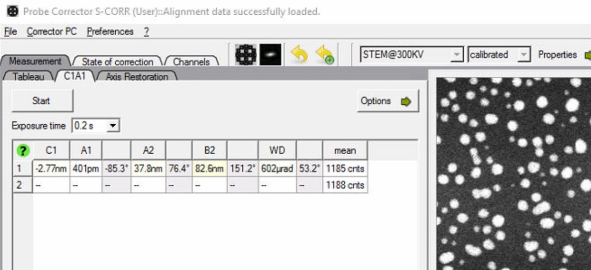
-
If
MC_STEM@300KVappears instead, the system is in monochromated STEM mode. Follow the steps below to reset to standard STEM mode. IfSTEM@300KVis displayed, skip ahead to “Configure C1A1 options.”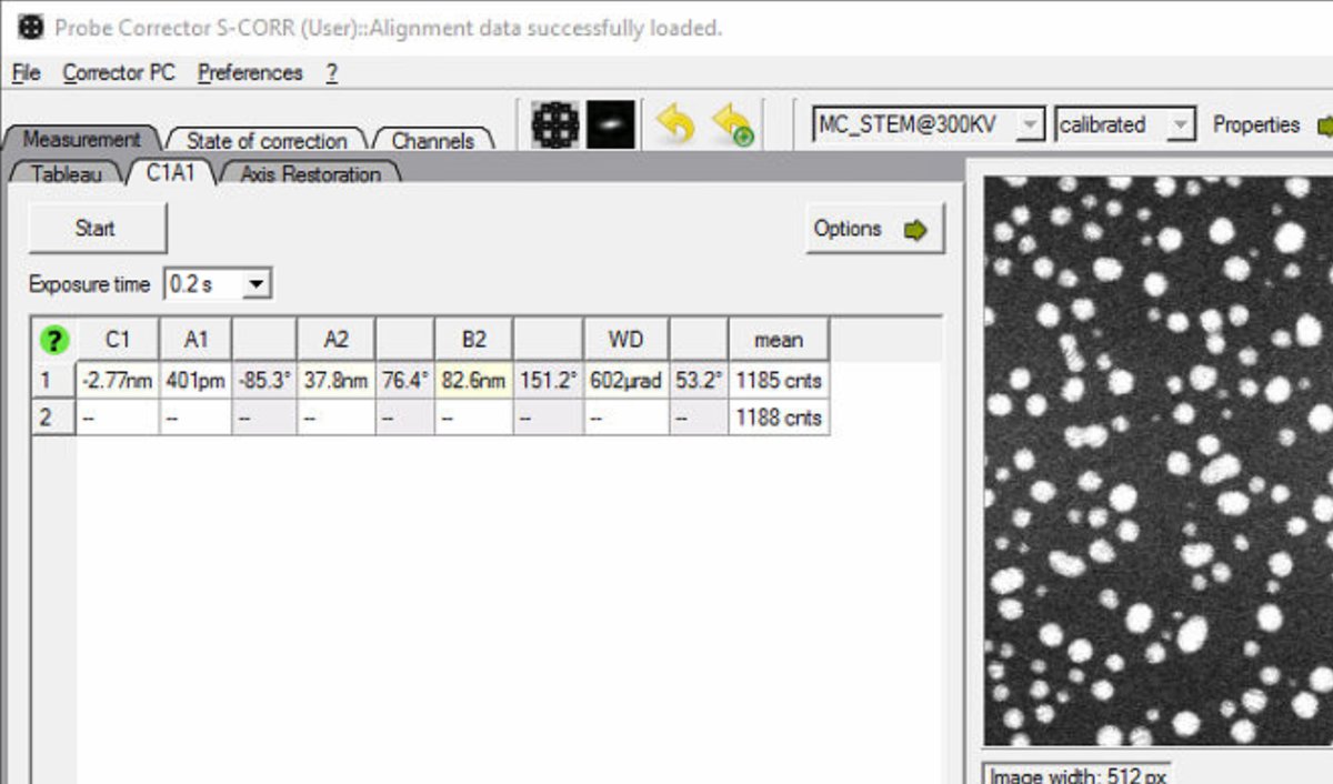
-
To reset, in TEMUI go to
Mono, then openMonochromator (Expert)and clickFilter: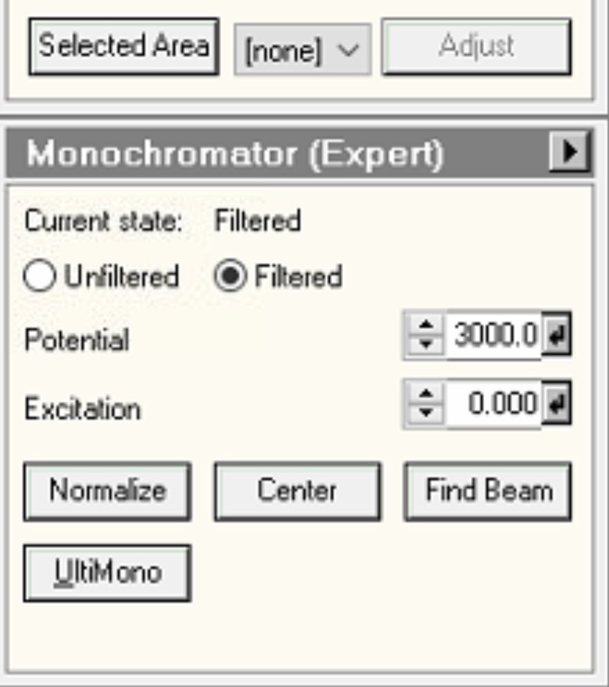
-
Then click
Unfilterto reset to standard STEM mode: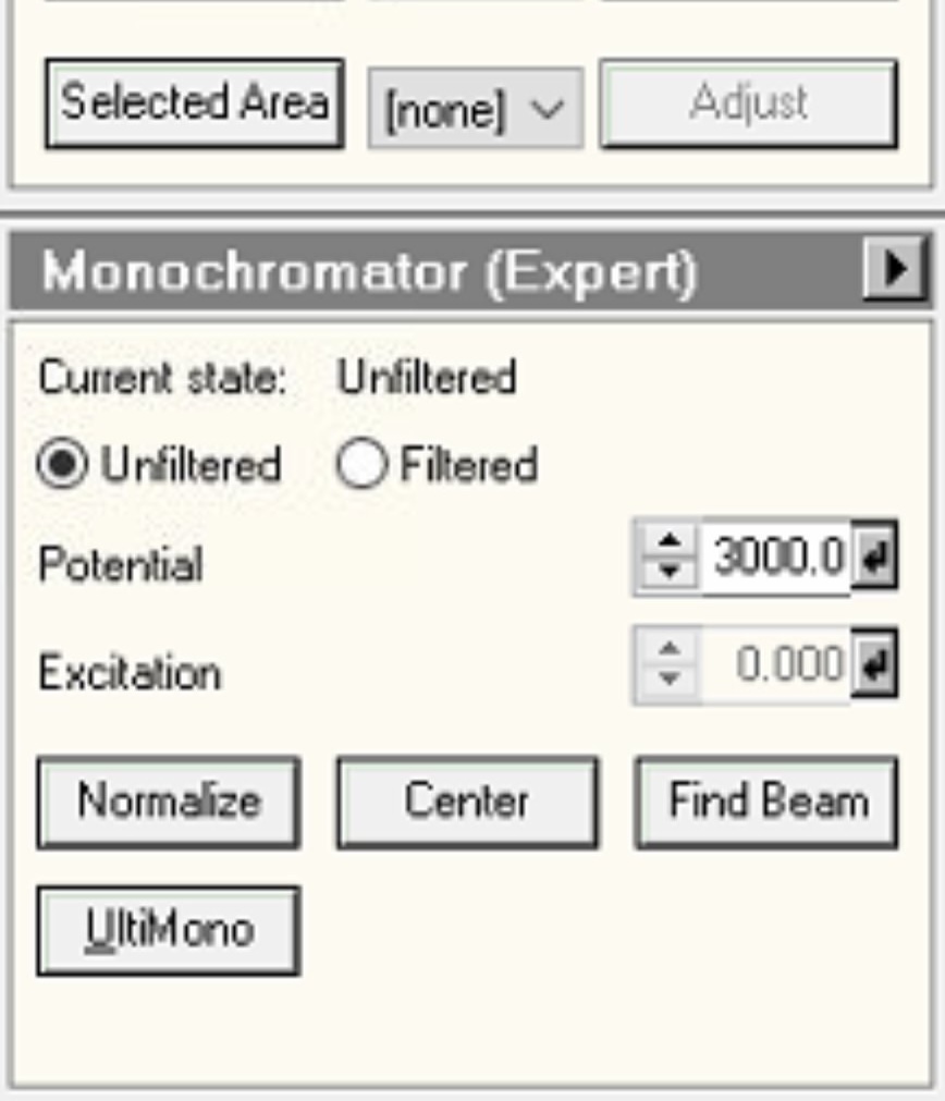
-
-
Configure C1A1 options
-
In the Probe Corrector software, click
Optionsto expand the configuration panel: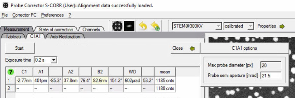
-
Set
Probe semi apertureto 30 mrad: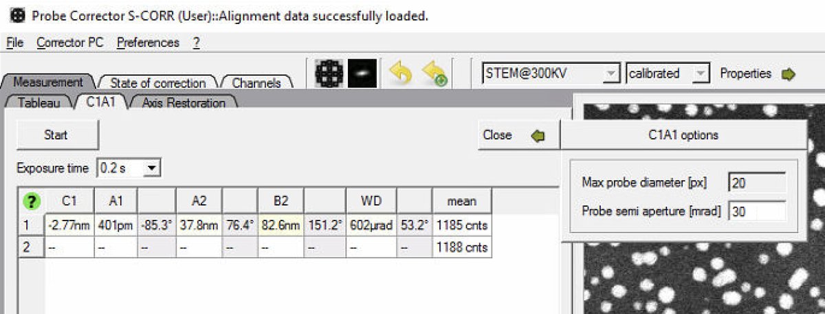
-
-
Switch to diffraction mode
-
Stop live scanning in
Veloxby clicking the play button, then ensureDiffractionmode is on on the hand panel. C1A1 analyzes the ronchigram, so diffraction mode (stationary probe) is required, not probe image mode (scanning):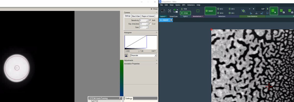
-
Click the
Beam Blankbutton to unblank the beam. Stopping the scan automatically blanks the beam. The Probe Corrector software requires an unblanked beam to read the ronchigram:
-
-
Run C1A1
-
Go to the
C1A1tab in theProbe Correctorsoftware. Before clicking Start, verify the ronchigram is visible on the left monitor: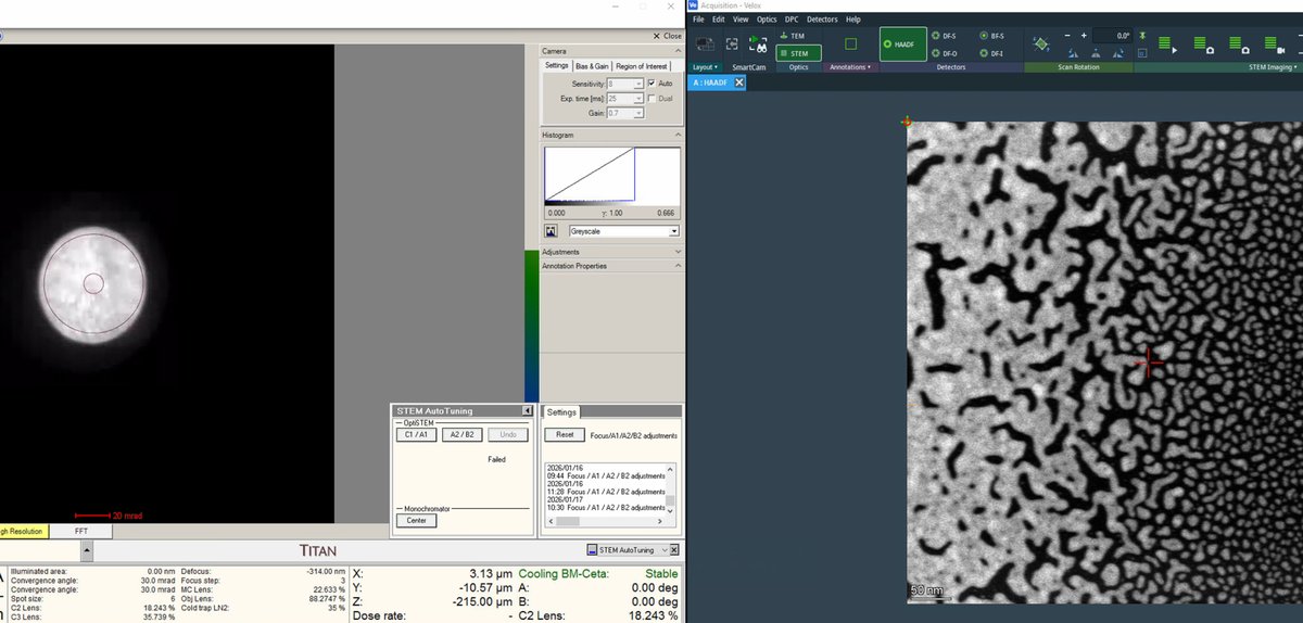
-
Click
Startto begin aberration measurement. The software continuously analyzes the ronchigram and displays measured aberration values (C1, A1, A2, B2, WD) in the table. -
Set Auto correct to 100% for the first iteration.
-
Click
0th-2ndto apply corrections for all first and second order aberrations.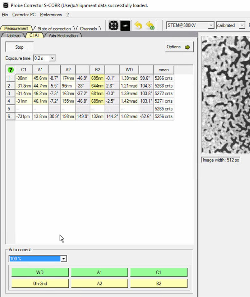
-
-
Iterate C1A1
-
Click
0th-2ndrepeatedly to apply corrections. Each row represents one measurement cycle. Watch the aberration values decrease with each iteration.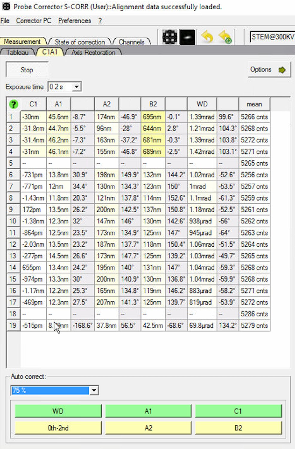
-
Reduce the Auto correct percentage to 75% after several iterations (typically 3 to 5) to prevent overcorrection.
If A1 is still high but other values are good, click
A1specifically to correct only astigmatism.
-
When to stop: C1A1 values are stable when they no longer decrease significantly between iterations. Target: C1 (defocus) < 1 nm and A1 (astigmatism) < 3 nm. Click
Stopwhen values are stable.
-
2.2 Tableau measurement
Tableau measures higher-order aberrations (A2, B2, C3, S3, A3) by acquiring ronchigram patterns at multiple beam tilt angles. The software analyzes how the ronchigram changes with tilt to extract the full aberration function. Tableau is more comprehensive than C1A1 and necessary for highest resolution.
-
Open Tableau tab
-
Switch to the
Tableautab in theProbe Correctorsoftware for full aberration measurement and correction. -
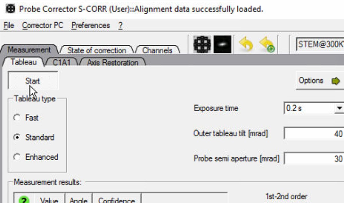
Select
Standardfor Tableau type. This acquires a sufficient number of tilt positions for accurate measurement without taking excessive time. -
Set the Outer tableau tilt to 40 mrad. Larger tilts probe higher-order aberrations but require more time.
-
Verify the Probe semi aperture is set to 30 mrad to match the beam settings.
-
Click
Optionsand select theA5toggle. It measures up to 5th order aberrations.
-
-
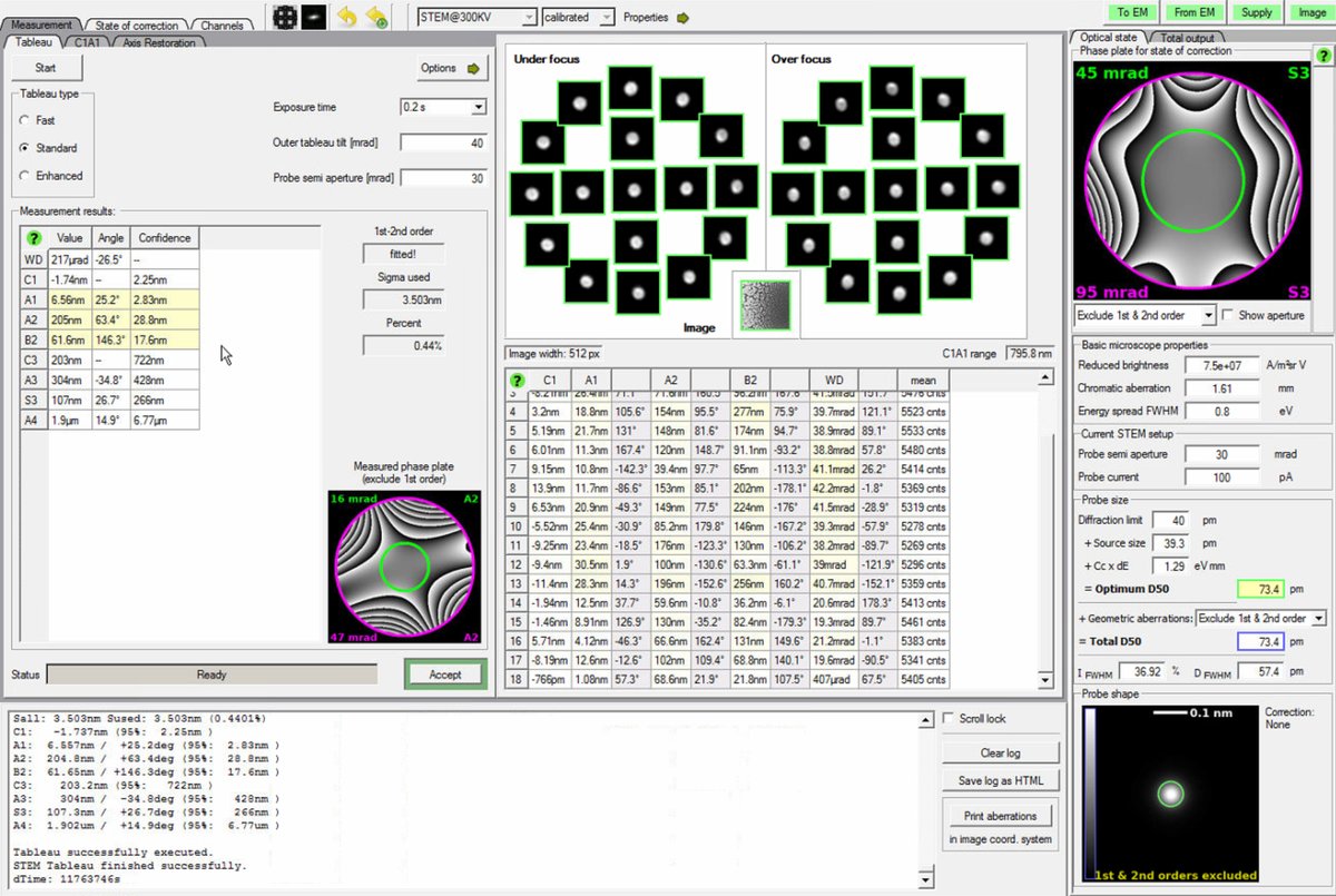
Run Tableau measurement
-
Click
Startto begin the Tableau measurement. The software automatically tilts the beam to multiple angles and acquires ronchigram images at each position. -
Wait for measurement completion. The ronchigram shifts across the screen as the software captures patterns at different tilts and focus levels (under-focus and over-focus at each tilt). This movement is expected.
-
Do not modify the stage position during measurement. If the beam is unstable, stop and ask staff.
-
-
Accept measurement
- Click
Acceptafter measurement completes. This validates the data for corrections.
- Click
-
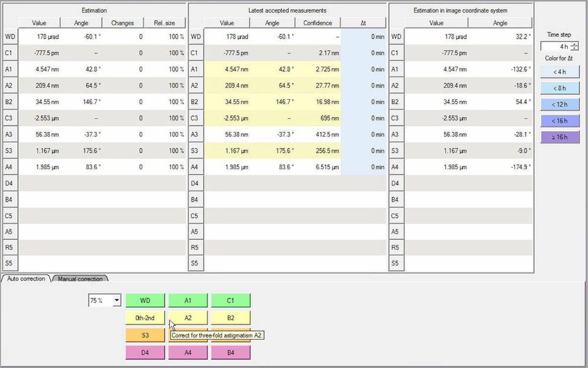
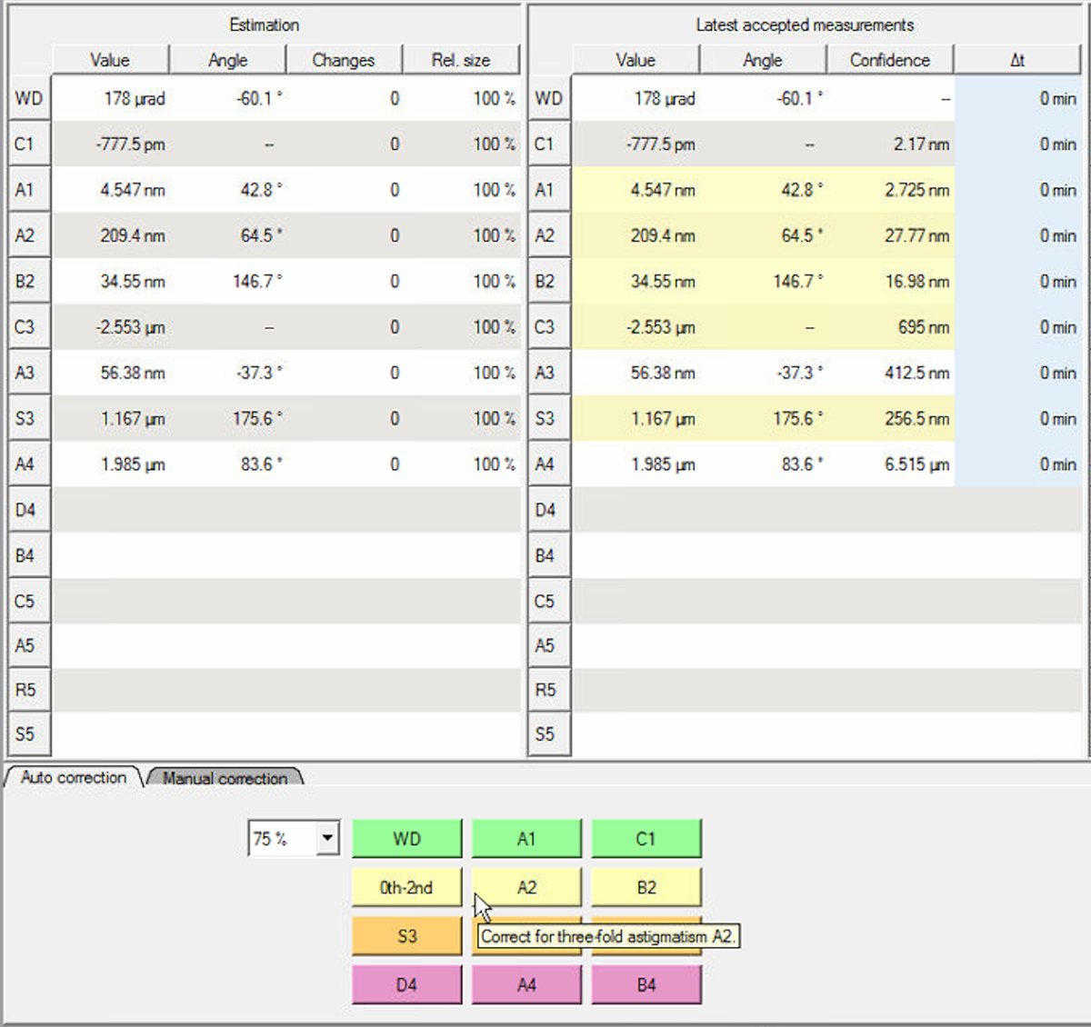
Review measurement results
-
Click the
State of correctiontab. This shows all measured aberration coefficients in three columns:- Estimation: Just measured values
- Latest accepted measurements: Previously applied corrections (yellow = outside limits)
- Estimation in image coordinate system: Values transformed to image coordinates
-
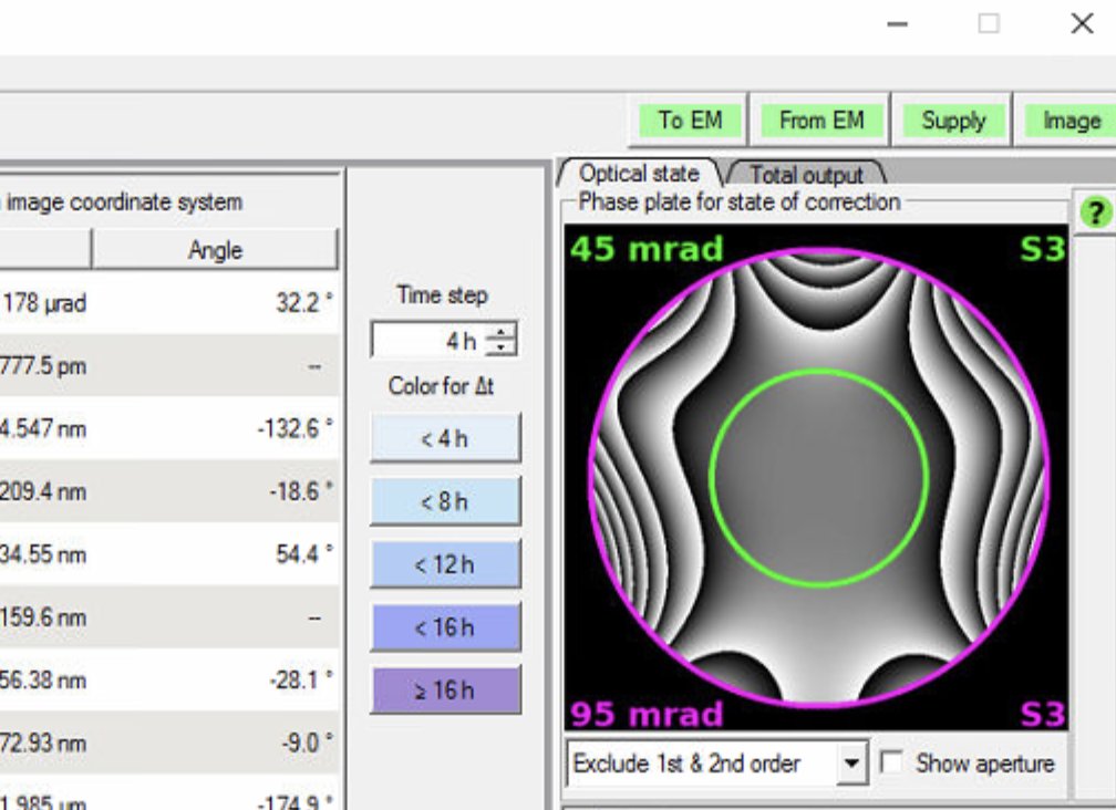
Check the phase plate visualization on the right. A well corrected probe has a flat, symmetric phase plate. Strong asymmetric patterns indicate uncorrected aberrations:
-
-
Apply corrections
-
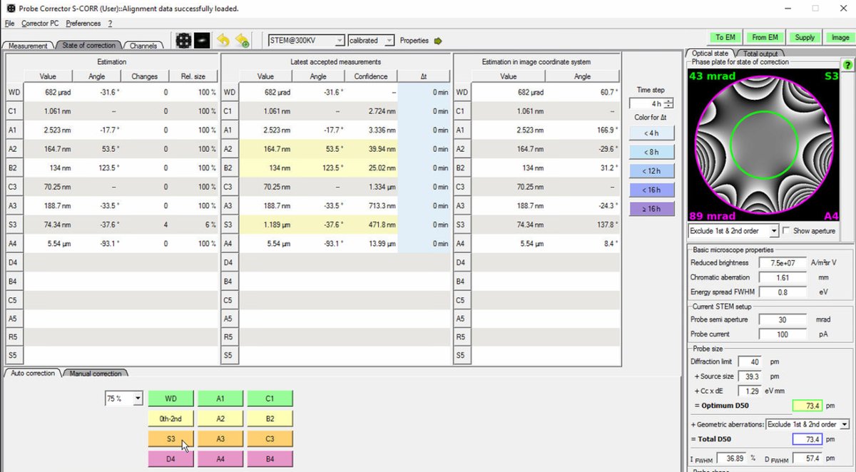
Set Auto correct to 75% to prevent overcorrection. Yellow highlighted values in the “Latest accepted measurements” column indicate aberrations outside acceptable limits. Correct these first. In this example, S3 (1.167 μm) and C3 (-2.553 μm) are highlighted yellow:
Note: either clicking
B4orD4can have a significant impact onC1andA1values.-
Click the aberration buttons at the bottom to apply corrections. The phase plate visualization shows the limiting aberration. Correct this one first. Click the button repeatedly until the value improves sufficiently, then move to the next limiting aberration.
-
The “Changes” column tracks how many corrections have been applied. After correcting S3 and C3, the values improve significantly:
- S3: 1.167 μm → 72.93 nm
- C3: -2.553 μm → -159.6 nm
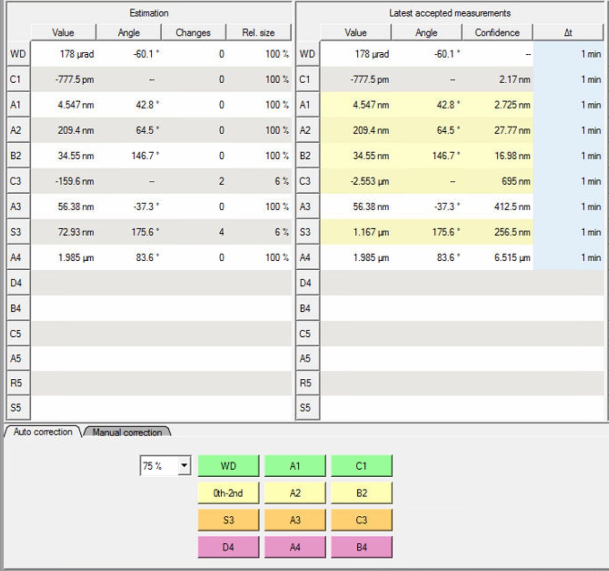
-
-
Run full measurement
-
After applying corrections, run another complete Tableau measurement to verify the improvements.
-
Check the aberration surface and phase plate displays. A well-corrected probe shows:
- Flat aberration surface with green in the center (minimal phase variation across the aperture)
- Symmetric phase plates without strong directional features
Target values (30 mrad semi-aperture):
Parameter Target C1 < 1 nm A1 < 3 nm A2 < 40 nm B2 < 25 nm C3 < 1.5 μm A3 < 1 μm S3 < 500 nm TODO: CONFIRM WITH ANDREW for IDEAL TOTAL D50
-
-
Verify with C1A1
- Return to the
C1A1tab in the Probe Corrector software. Tableau correction can sometimes introduce small first-order errors. - Click
Startto begin C1A1 measurement again. - Click
A1to correct any residual astigmatism introduced by Tableau. - Click
0th-2ndif defocus also needs adjustment. - Iterate between Tableau and C1A1 if necessary until all values are within specification.
- Return to the
-
Check resolution
-
The
State of correctionpanel displays resolution estimates on the right side: Total D50 and Optimum D50. D50 represents the probe diameter containing 50% of the beam intensity (smaller = better resolution).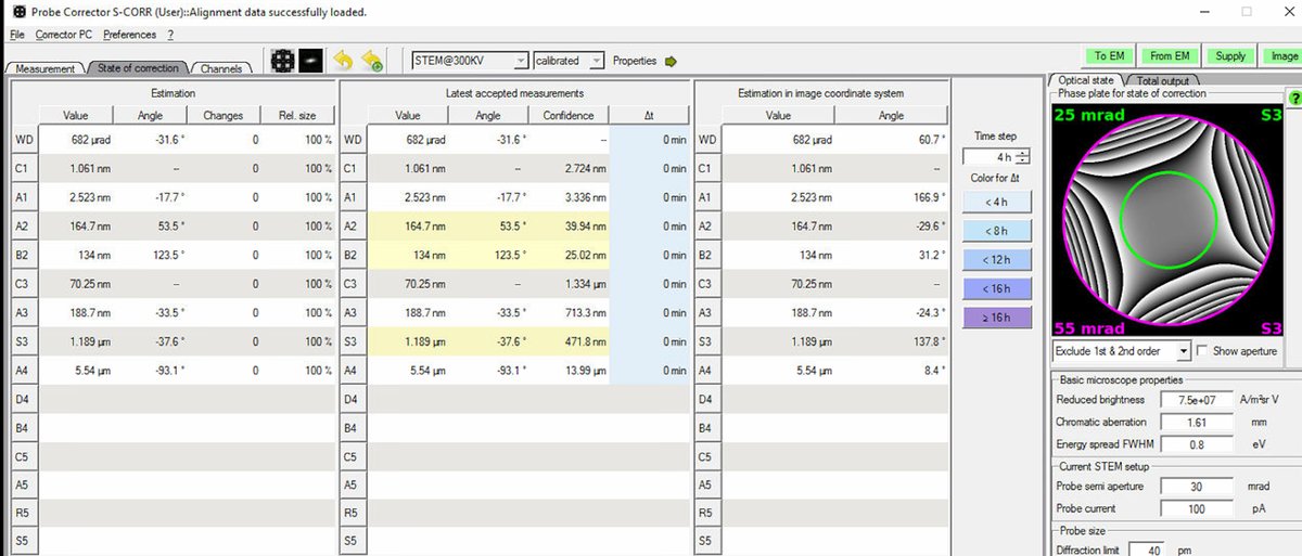
TODO: CONFIRM WITH ANDREW
-
Target: Total D50 of 70-75 pm for high-resolution STEM imaging. The Optimum D50 shows the theoretical best achievable with current aberrations. If these values match closely, corrections are complete.
-
If D50 values are significantly higher than target, continue iterating: run another Tableau measurement, apply corrections, then verify with C1A1. The image below shows C1A1 iterations after Tableau corrections:
-
-
Return to probe image mode
- Once correction is complete, press the
Diffractionbutton on the hand panel to switch back to probe image mode (STEM scanning). - The system is now ready for high-resolution image acquisition.
- Once correction is complete, press the
Part 3: Imaging
3.1 Acquire images
With aberration correction complete, the system is ready for high-resolution STEM image acquisition. The probe is optimized for atomic-resolution imaging.
-
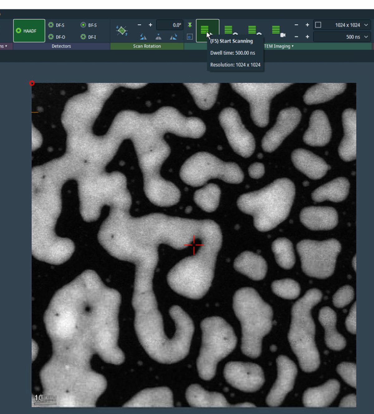
Acquire HAADF image
-
In
Velox, clickSTEMto enter STEM mode, then clickHAADFto select the HAADF detector. -
Click the play button to start live scanning. Image quality is noticeably improved compared to before correction. A well-corrected probe produces sharper, more detailed images.
-
For initial survey imaging, set resolution to 1024×1024 and dwell time to 500 ns. Fast scanning enables navigation while maintaining image quality.
-
-
Navigate to area of interest
-
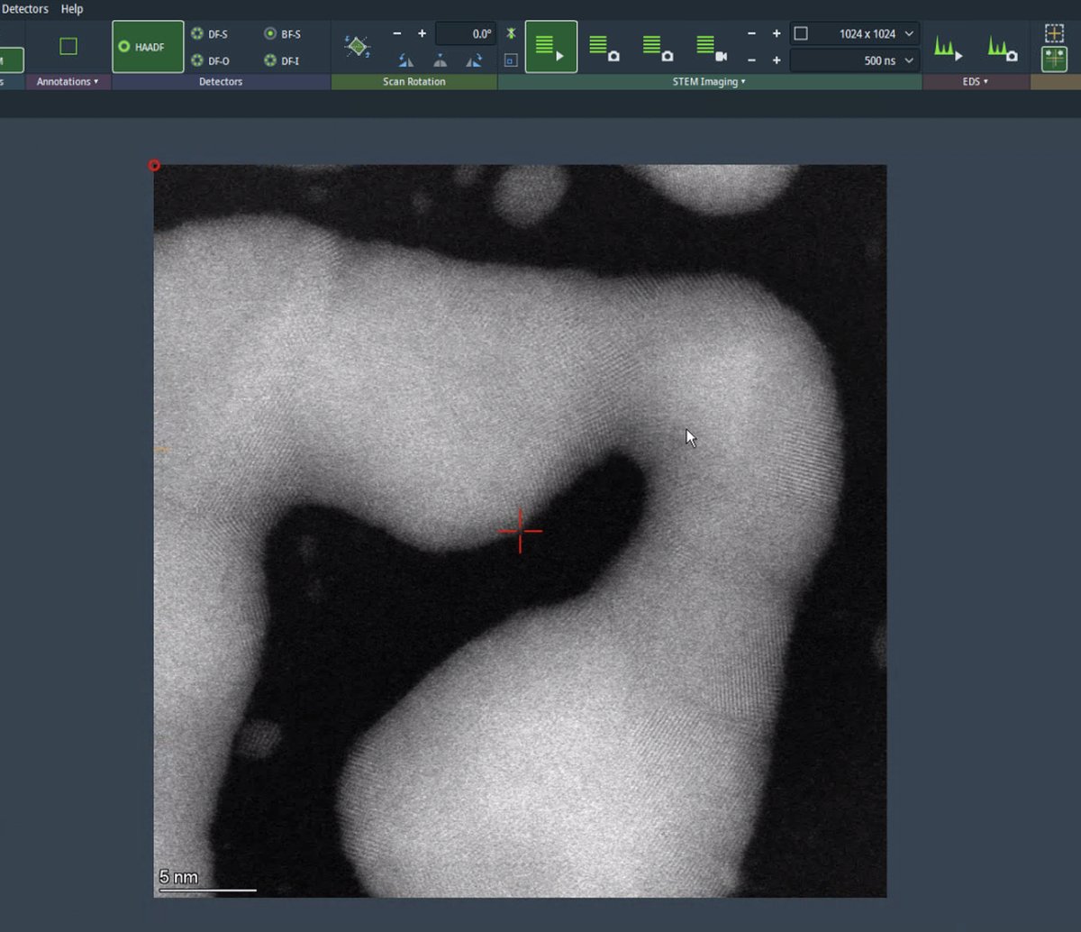
Use the live scan to find the region of interest. Use the joystick or click on the image to move to different regions. With a well-corrected probe, atomic lattice fringes are visible in crystalline materials.
-
Adjust focus using the z-height controls if needed. Small focus changes can significantly affect atomic-resolution contrast.
-
-
Capture high-resolution scan
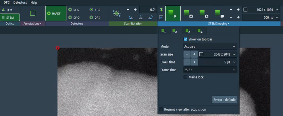
-
Increase the resolution to 2048×2048 or higher. Check the Velox toolbar to verify resolution and dwell time settings before starting the acquisition.
-
Increase the dwell time to 5 µs for better signal-to-noise ratio. Longer dwell times collect more electrons per pixel, reducing noise but increasing total scan time and potential for drift artifacts. After acquisition completes, the beam is blanked automatically to prevent sample damage.
-
3.2 Fine-tuning with Sherpa
Sherpa provides rapid aberration correction that is faster than full Tableau measurement. Use Sherpa for quick refinements after the main alignment, or when aberrations drift during extended imaging sessions.
-
Prepare for Sherpa
-
Before running Sherpa, verify the ronchigram is centered. Press the
Diffractionbutton on the hand panel to switch to diffraction mode (view the ronchigram). -
In
TEMUI, go toDirect Alignmentsand selectDiffraction Shift and Focus alignment: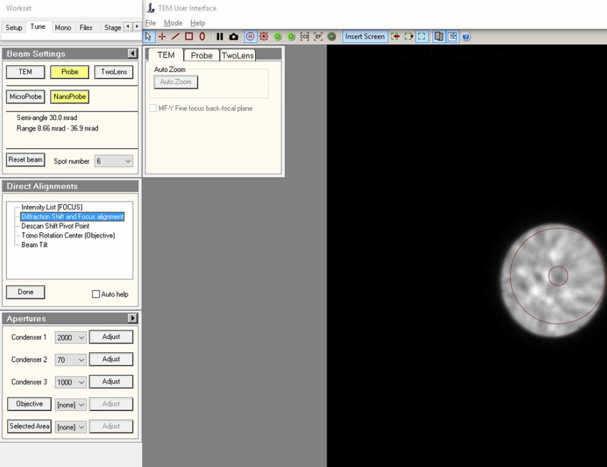
-
Use the
mulXYknobs to center the ronchigram on the display. A centered ronchigram ensures Sherpa measurements are accurate.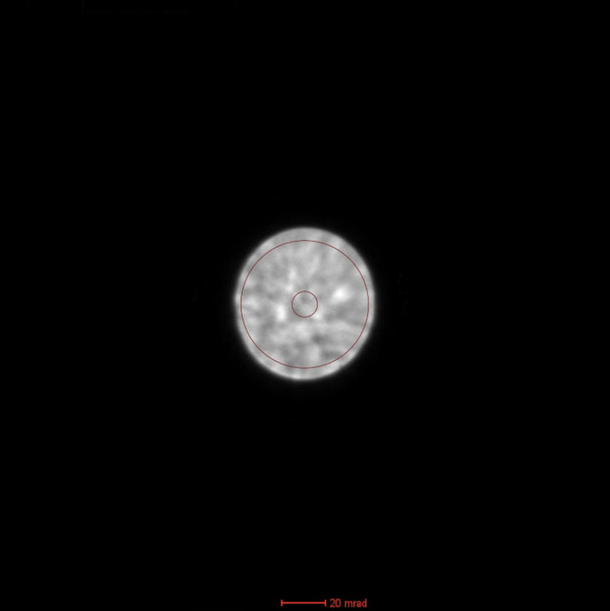
-
-
Adjust C2 aperture (optional)
-
To change C2 aperture size (for example, switching to 50 µm for different probe conditions), locate the
Aperturespanel and change Condenser 2 from 70 to 50 (or the desired size).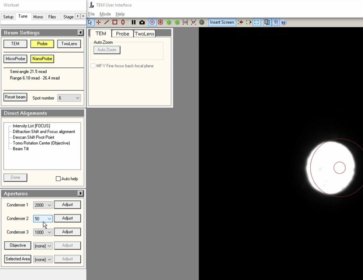
-
Click
Adjustto center the new aperture. The beam remains centered when changing aperture sizes. If not centered, use the adjustment controls to re-center.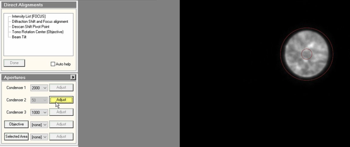
-
-
Open Sherpa
-
Open the
Sherpasoftware. Sherpa displays the HAADF image with a crosshair marker indicating the measurement region.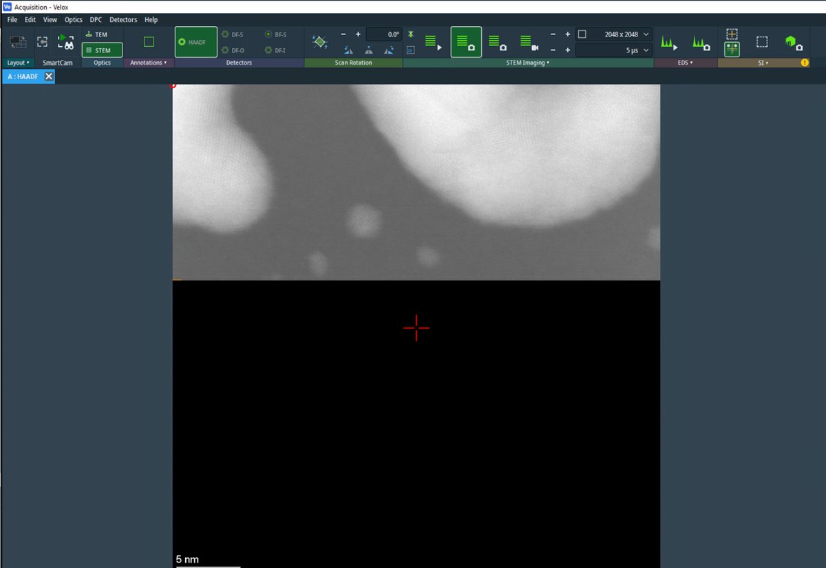
-
Click
C1/A1to run first-order correction (defocus and 2-fold astigmatism).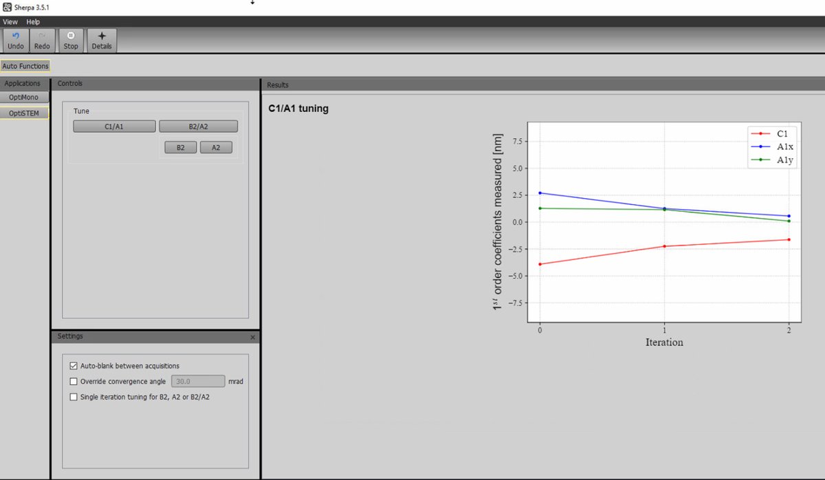
-
-
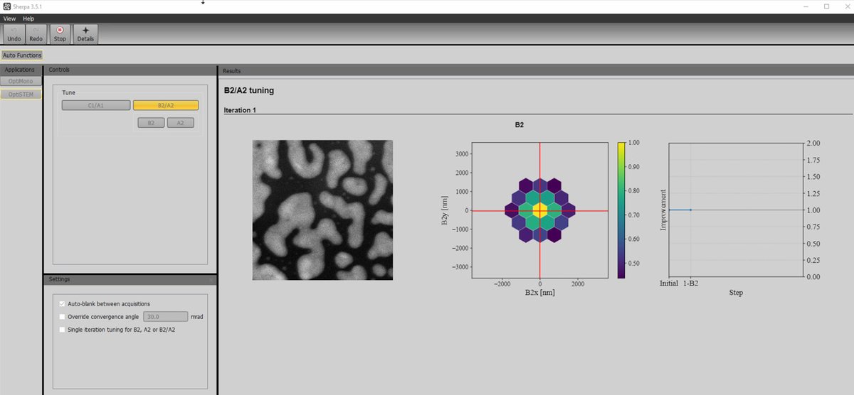
Run B2/A2 tuning
-
After C1/A1 completes, click the
B2/A2button to correct second-order aberrations (axial coma B2 and 3-fold astigmatism A2). -
Wait for the tuning to complete. Sherpa acquires images and determines optimal corrections.
-
Run multiple iterations if the first pass does not achieve optimal results.
-
-
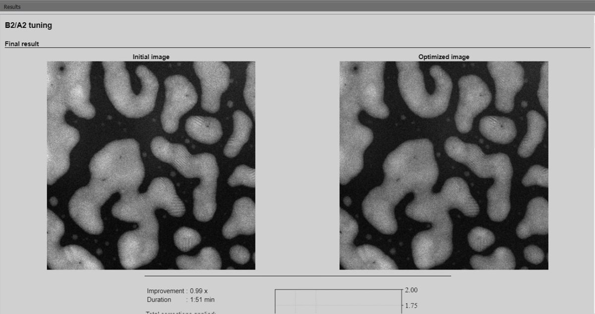
Review results
-
Sherpa displays the initial image alongside the optimized image for comparison. The corrected image shows improved sharpness and resolution.
-
3.3 Load your own sample
After completing probe correction on the standard sample, follow the below steps unload the current sample standard and load your own. For holder-specific instructions (single-tilt, double-tilt, tomography), see Sample Loading.
-
Remove the standard sample
-
Put on gloves before handling any holders or samples.
-
Blank the beam and verify the screen is inserted. The screen protects the detectors and cameras below from the beam.
-
Close the column valves by pressing
Column Valves Closed.If a “VCP” error occurs, follow the instructions on the Spectra NEMO page.
-
Reset the holder by clicking
reseton theStagemenu.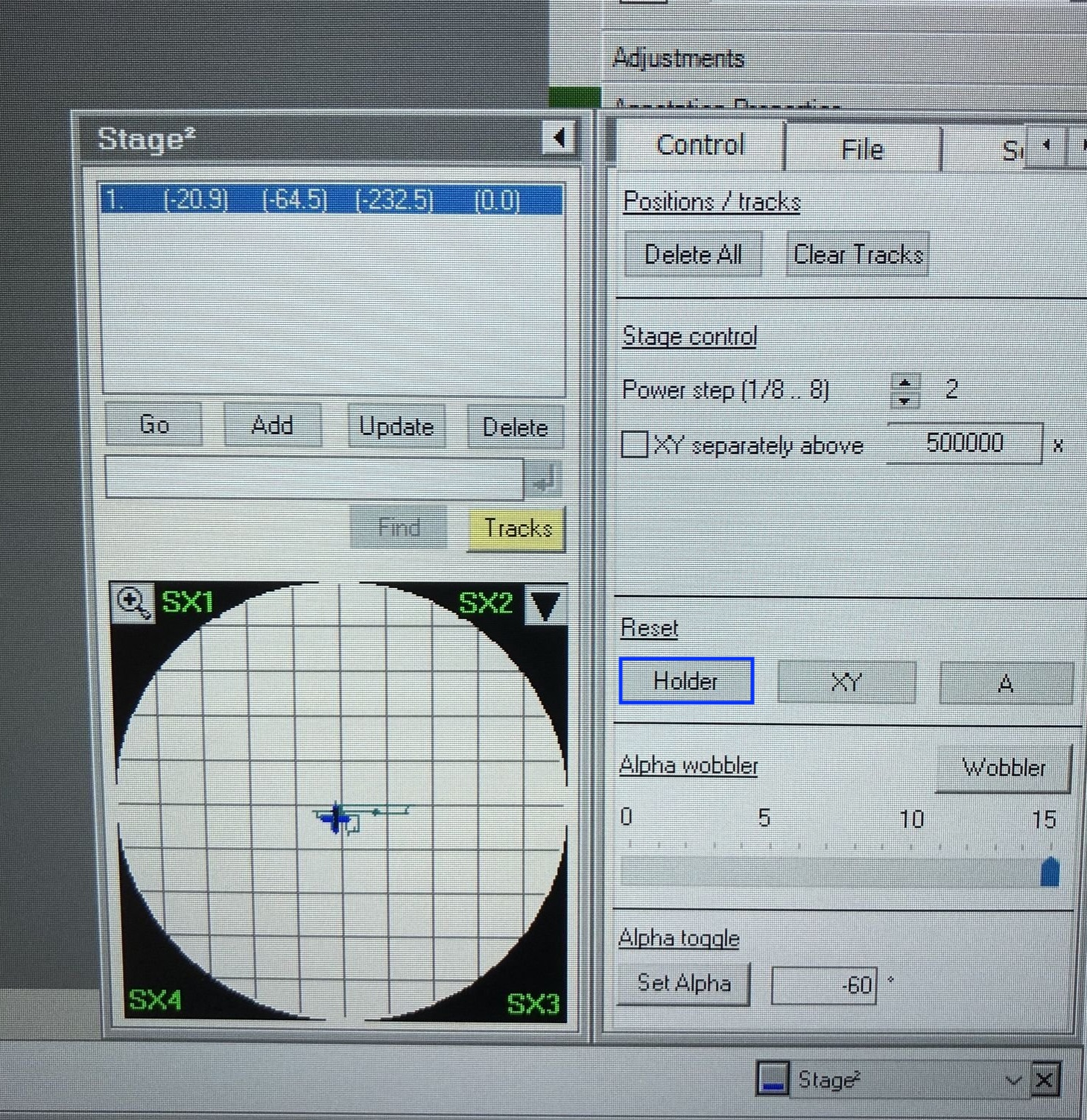
-
Confirm the stage x, y, z values are returning to zero after you reset the holder stage.
-
Pull the holder straight out to the first resistance point. Do not force beyond this point. Turn clockwise, then pull the rest of the holder out continuously.
-
-
Load your sample and insert the holder
IMPORTANT: Do not remove the standard sample from the single-tilt holder. Use a separate holder to load your sample.
-
For holder-specific loading instructions, see Sample Loading.
-
Align the holder with the blue line on the goniometer.
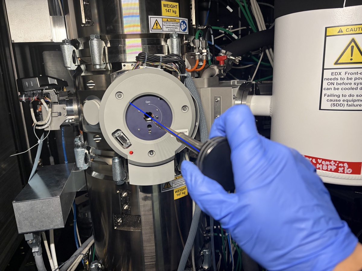
-
Push the holder in until you feel resistance. Do not push all the way in.
-
The turbo pump starts automatically. Wait ~2 minutes for pressure to stabilize. You can monitor the time in
TEMUIor on the screen attached to the Spectra instrument.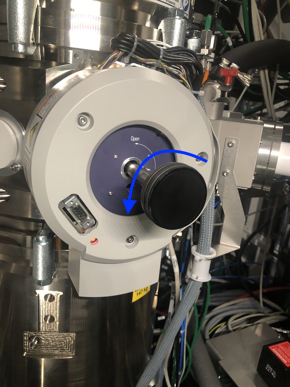
Why wait? The holder insertion opens a small chamber to atmosphere. The turbo pump must evacuate this air before you can insert the holder into the main column. Rushing this step would introduce air into the ultra-high vacuum column, potentially damaging the electron gun and contaminating the system.
-
Wait until the PPII gauge drops into the high 10⁻⁶ mbar to low 10⁻⁷ mbar range before continuing. PPII reads the load lock / projection chamber pressure; the holder insertion path is only safe to advance once PPII has reached this range.
NOTE: In the example above PPII reads 7.39 × 10⁻⁶ mbar (high 10⁻⁶ range), which is right at the threshold. Wait until it drops further (low 10⁻⁶ or into 10⁻⁷) for a more conservative margin before the next step.
-
Turn the holder counter-clockwise until you feel gently stuck, then guide the holder to push in. The holder should move in smoothly.
-
In
TEMUI, turn off the turbo pump. Confirm the holder type when prompted.
-
Re-do eucentric height
- Open column valves and re-do eucentric height for your new sample (1.3). Each sample sits at a different physical height in the holder. Find the ronchigram “blow-up” point again so the sample stays centered when tilted and the probe is properly focused.
- Run a quick C1A1 or Sherpa to verify probe correction still holds after the sample change. For beam-sensitive or low-contrast samples where Sherpa cannot be used, see Manual Aberration Correction (Advanced).
Part 4: End session
4.1 Reload the standard sample
-
Reload the standard sample
-
Put on gloves before handling any holders or samples.
-
Blank the beam and verify the screen is inserted.
-
In
TEMUI, clickColumn Valves Closed. -
Click
Reset Holderunder theStagemenu. Visually verify that the X, Y, and Z stage coordinates are reset after the button is pressed.
-
Pull the holder with your sample straight out to the first resistance point. Do not force beyond this point. Turn clockwise, then pull the rest of the holder out continuously.
-
Set aside your holder and pick up the single-tilt holder with the standard sample.
-
Push the single-tilt holder with the standard sample in until you feel resistance. Do not push all the way in.
-
The turbo pump starts automatically. Wait ~2 minutes for pressure to stabilize.
-
Turn the holder counter-clockwise until you feel gently stuck, then guide the holder to push in.
-
In
TEMUI, turn off the turbo pump. ConfirmSingle tilton TEMUI.
-
4.2 Checklist before leaving the Spectra room
- Beam is blanked.
-
Reset Holderhas been pressed and X, Y, Z stage coordinates are verified reset. - Stage is returned to 0° tilt (alpha and beta).
- Arina detector is retracted, verified on the left hand panel.
- Arina detector is turned off, verified on the local Firefox URL.
-
INT SCANphysical button is in pressed state. - Screen is inserted.
- Column valve is closed.
- Turbo pump is turned off.
- Standard sample is loaded.
- All holders are capped and stored in the holder box.
- The sample loading area is tidy.
- Spectra usage is terminated on NEMO.
- Internet accounts (Google, Outlook, etc.) are signed off.
- Fill out the logbook if anything unusual happened during the session.
Troubleshooting
Common problems encountered during STEM sessions.
| Problem | Cause | Solution |
|---|---|---|
| Image drifts when tilting | Eucentric height not set | Re-do eucentric height after loading a new sample |
| C1A1 measurements unstable or fail | Velox is still scanning | Stop live scanning in Velox before running C1A1, then verify the beam is unblanked |
| Aberration values oscillate instead of converging | Overcorrection percentage too high | Start with 100% Auto correct, reduce to 75% as values approach target |
| C1A1 or Tableau shows no signal | Beam is blanked | Click Beam Blank button to unblank before running aberration measurements |
| Good Tableau values but poor image resolution | Missing C1A1 verification step | After Tableau, always run C1A1 again to fine-tune defocus and astigmatism |
| Beam disappears from view | Random adjustments displaced the beam | Go to lower magnification until beam is visible, use joystick to move sample to center, then go to Diffraction Shift and use mulXY to center the beam |
| Lost beam or need to redo alignment | Column misalignment after extended session | Redo eucentric height (1.3) and monochromator tune (1.6). If you cannot find the sample, switch to TEM mode for easier navigation (TEM Spectra) |
FAQ
Beam blanking
When the beam is blanked, the electron beam is deflected away from the sample so no electrons hit it. This prevents unnecessary radiation damage to the sample when not actively imaging. The beam is automatically blanked when scanning stops or after taking a picture. Manual blank/unblank is available via the Beam Blank button on the hand panel or in the software.
Monochromator focus adjustment
The monochromator filters the energy spread of the electron beam by passing it through a narrow slit. Setting Focus = 0 places the beam crossover exactly at the monochromator slit plane. This position maximizes electron throughput while maintaining energy filtering. If the focus is offset from zero, the beam crossover occurs before or after the slit, reducing beam current and degrading energy resolution.
Appendix
Aberration notation
Different notations exist for aberrations in the literature. The table below shows the Krivanek notation (used in Probe Corrector software), the alternative notation (used in this guide), and descriptions.
| Krivanek | Alt | Description | Krivanek | Alt | Description |
|---|---|---|---|---|---|
| \(C_{10}\) | \(C_1\) | Defocus | \(C_{41}\) | \(B_4\) | 4th order coma |
| \(C_{12}\) | \(A_1\) | 2-fold astigmatism | \(C_{43}\) | \(D_4\) | 3-lobe aberration |
| \(C_{21}\) | \(B_2\) | Axial coma | \(C_{45}\) | \(A_4\) | 5-fold astigmatism |
| \(C_{23}\) | \(A_2\) | 3-fold astigmatism | \(C_{50}\) | \(C_5\) | 5th order spherical |
| \(C_{30}\) | \(C_3\)/\(C_s\) | Spherical | \(C_{52}\) | \(S_5\) | 5th order star |
| \(C_{32}\) | \(S_3\) | Star aberration | \(C_{54}\) | \(R_5\) | Rosette |
| \(C_{34}\) | \(A_3\) | 4-fold astigmatism | \(C_{56}\) | \(A_5\) | 6-fold astigmatism |
Changelog
- May 6, 2026 - Promote End session to Part 4 and add it to the overview table
- Mar 1, 2026 - Add pre-session checklist, sample loading section with glove requirement, end session with explicit reload steps, fix image paths
- Feb 28, 2026 - Add prerequisite link to TEM Alignment guide; add lost-beam troubleshooting
- Jan 31, 2026 - Initial draft: instructions by Sangjoon Bob Lee, screenshots by Andrew Barnum during Spectra 300 hands-on training
Manual aberration correction (advanced)
Caution
VERY ROUGH DRAFT - This guide is a collection of open questions and procedures to be verified during future practice sessions.
TODO: Replace with real screenshots from a manual correction session on a beam-sensitive sample.
This guide covers manual aberration correction without Sherpa on the Spectra 300. Sherpa is an automated aberration correction tool that works well on high-contrast samples like gold nanoparticles (see Fine-tuning with Sherpa in the STEM guide). However, manual correction is necessary when:
- Beam-sensitive samples: Sherpa’s iterative scanning damages the sample before correction completes (e.g., organic or biological specimens).
- Low-contrast samples: Sherpa relies on image contrast to measure aberrations. If the sample has insufficient contrast, Sherpa cannot converge on a solution.
Prerequisite: Complete the STEM alignment through Part 2 (probe correction on the gold standard sample) before attempting manual correction on your own sample.
For an interactive visualization of how aberrations affect the ronchigram, see the Ronchigram Simulator.
Acronyms:
mulXY- Multifunction X/Y knobs on hand panelTEMUI- TEM User Interface (software)A1- Twofold astigmatism (probe stretched into an ellipse)A2- Threefold astigmatism (triangular probe distortion)B2- Axial coma (asymmetric “comet tail” probe shape)
Before you start
This guide assumes you have already completed Part 2: Probe Correction on the gold standard sample and loaded your own sample. The probe correction from the gold standard should largely carry over. However, sample loading and stage movement introduce small aberrations that need manual correction on your sample.
-
Find your sample region
- Load your sample following Sample loading.
- Find your region of interest. After stage movement, wait ~5 min for mechanical stabilization before correcting aberrations.
Two methods for manual correction
There are two independent methods to manually adjust aberrations. They use separate software and do not communicate with each other: changes in one are not reflected in the other. Use whichever method is more appropriate for your situation, or combine both.
Method 1: Probe Corrector | Method 2: Stigmator (TEMUI) | |
|---|---|---|
| Software | Probe Corrector S-CORR (top left monitor) | TEMUI + hand panel |
| Where in column | Aberration corrector multipoles | Condenser lens system (above the corrector) |
| Controls | Arrow keys + Multiplier | mulXY knobs |
| Aberrations | All (A1, A2, B2, C3, etc.) | A1, Condenser stigmator, B2, etc. |
| Feedback | Aberration table + ronchigram | Ronchigram only |
Method 1: Probe Corrector software
-
Adjust aberrations in Manual correction
-
In the
Probe Correctorsoftware, click theState of correctiontab, then clickManual correction. -
Select an aberration parameter (e.g.,
AT_A1is selected in the image) and use the left and right arrow keys to adjust its value. Use theMultiplierto change the step size. Watch the ronchigram on the bottom monitor for live feedback as you adjust.
TODO: Define what “good” looks like without Sherpa. Determine criteria for the ronchigram, FFT, and probe shape.
-
Method 2: Stigmator via TEMUI and hand panel
-
Adjust aberrations with the hand panel
TODO: Verify the full procedure and which aberrations can be corrected via
TEMUI(A1, Condenser stig, B2, etc.).-
Press the
Stigmatorbutton on the hand panel. -
When
Stigmatoris selected, the ronchigram automatically zooms in and out (the system oscillates the stigmator to show the effect). Adjust themulXYknobs to make the ronchigram more circular (symmetric in both X and Y).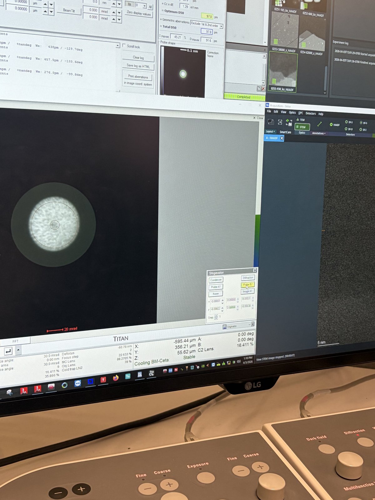
-
Verify final correction
-
Check correction quality
-
Check the live FFT of the HAADF image. Rings should be round, not streaked.
-
Switch to diffraction mode to view the ronchigram. The featureless central region should be circular and as large as possible. If it is elliptical, A1 still needs correction. If it is shifted to one side, B2 needs correction.
TODO: What is the minimum correction quality needed for atomic resolution on beam-sensitive samples?
-
End session
Follow the steps in End session from the Spectra STEM guide.
Acknowledgments
Thank you to Parivash Moradifar for allowing @bobleesj to shadow her session and for teaching the manual correction workflow. Images captured during her session.
Changelog
- Apr 3, 2026 - Initial draft with open questions by @bobleesj
Spectra 300 maintenance (DRAFT)
This page collects recovery and maintenance procedures specific to the Spectra 300 at Stanford SNSF. These are not part of normal acquisition but may be needed mid-session. Drafted by Sangjoon Bob Lee from staff-provided notes and images.
Caution
This is a rough draft. Confirm each procedure with staff before relying on it.
Overview
| Procedure | When to use | Time |
|---|---|---|
| Liquid nitrogen fill | LN dewar reads low during session | 10-15 min |
| Octagon recovery | TEMUI shows an Octagon vacuum error | 2-5 min |
Liquid nitrogen fill
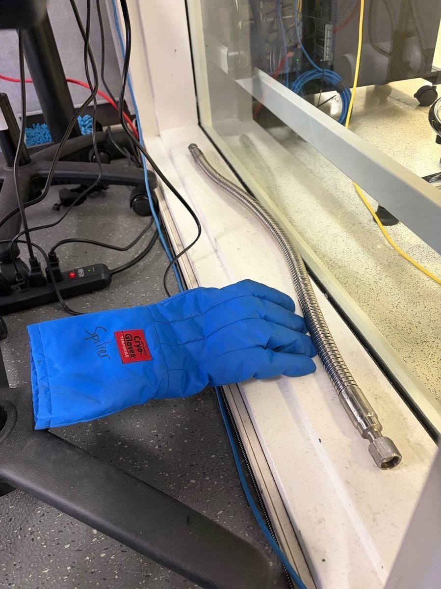
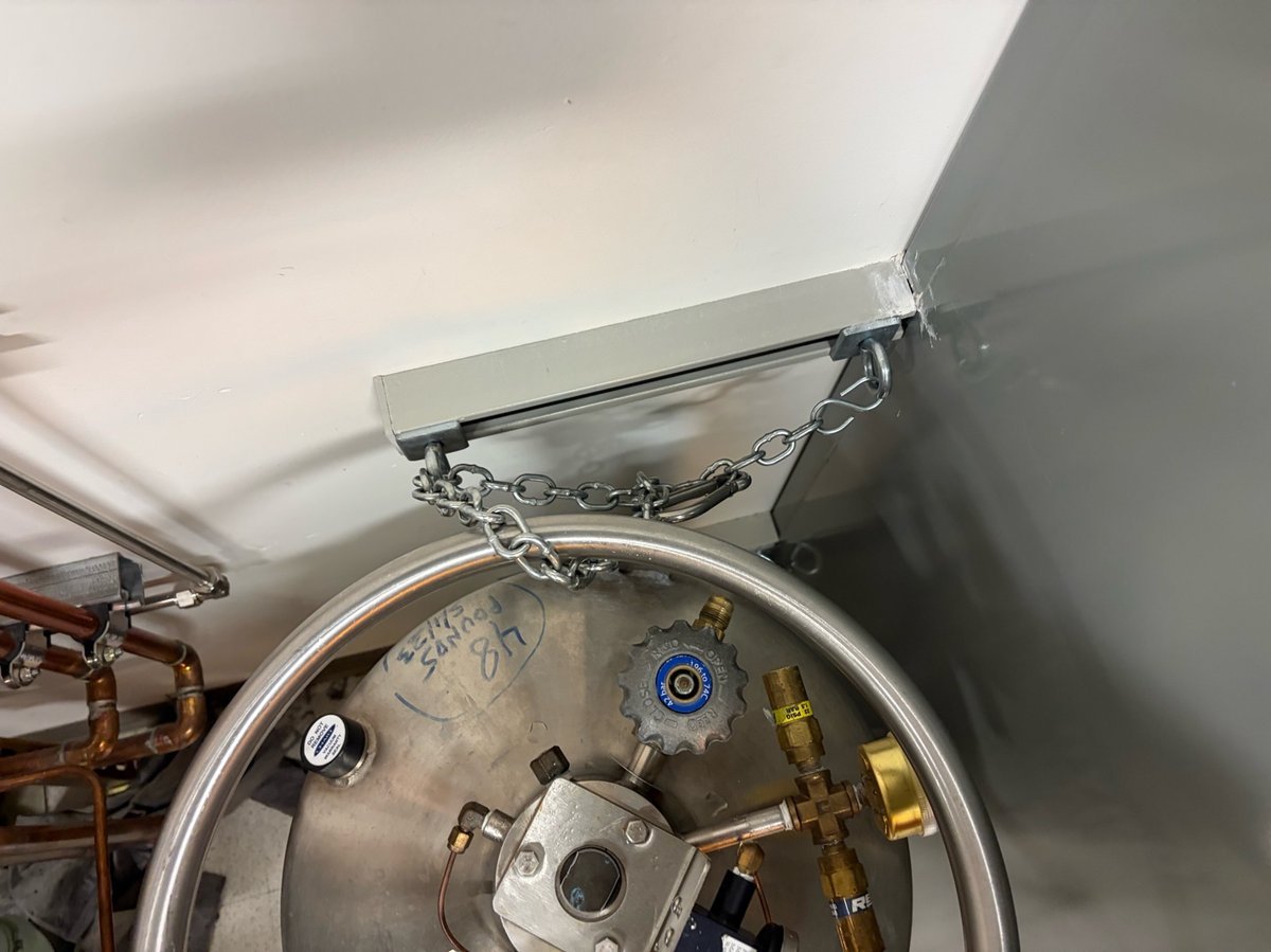
Refill the LN dewar from the portable nitrogen tank in the back room when the level drops. Wear cryo gloves — liquid nitrogen can cause severe cold burns.
TODO: Confirm at what nitrogen level (%) staff want users to start a refill.
-
Check the nitrogen level
-
On the Spectra touch panel, check the
Nitrogen Levelreadout. Refill when the level reads low.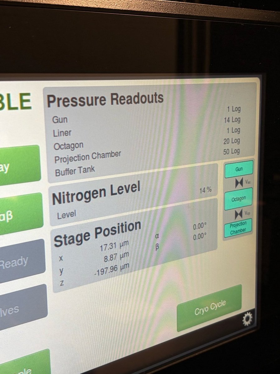
-
-
Bring the portable tank into the Spectra room
-
The portable nitrogen tank is stored in the back room.
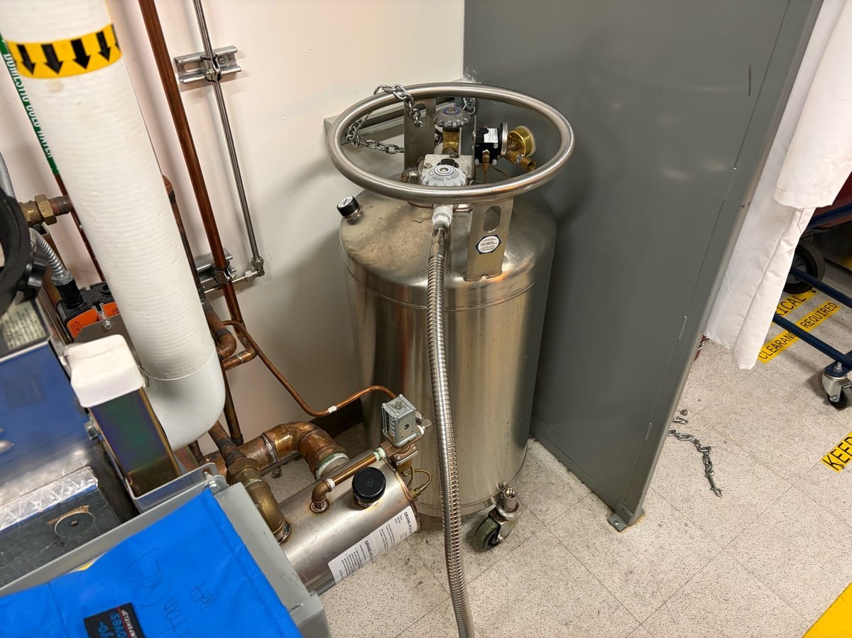
-
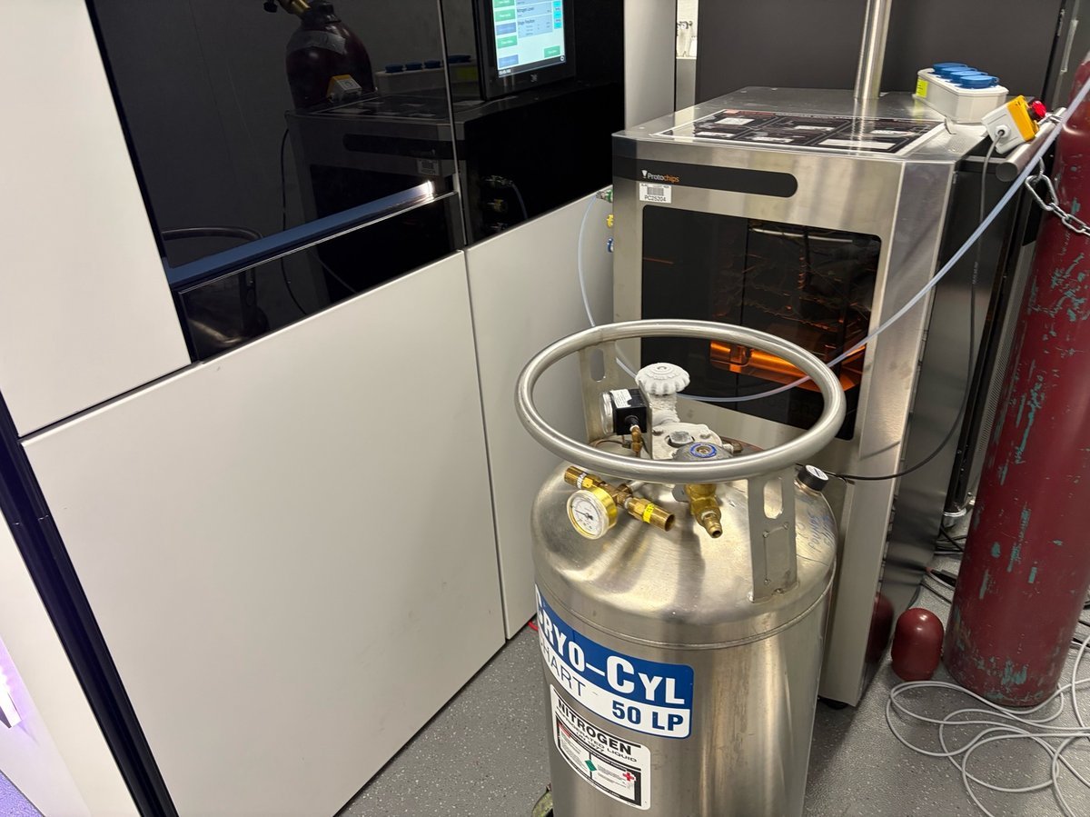
Roll the tank to the sample-loading area inside the Spectra room.
-
-
Put on cryo gloves
-
Cryo gloves and the transfer hose are stored near the sample-loading zone.
-
-
Connect the transfer hose
-
On the portable tank, identify the valve labeled
LIQUID. The other valve is for gas — do not use it.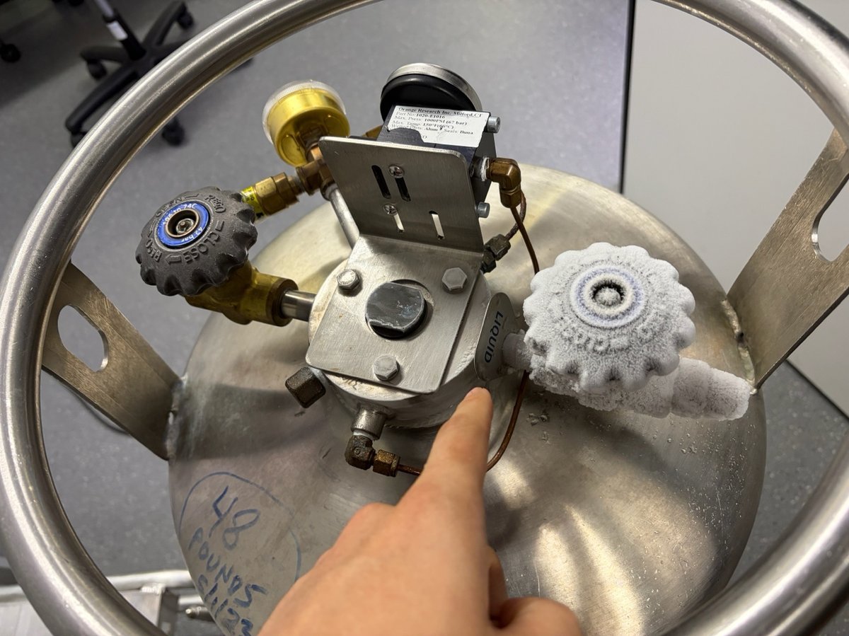
-
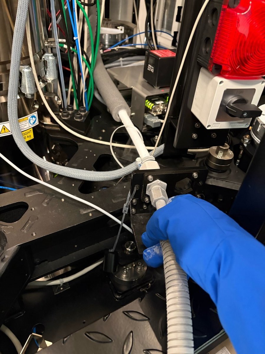
Attach one end of the transfer hose to the
LIQUIDvalve.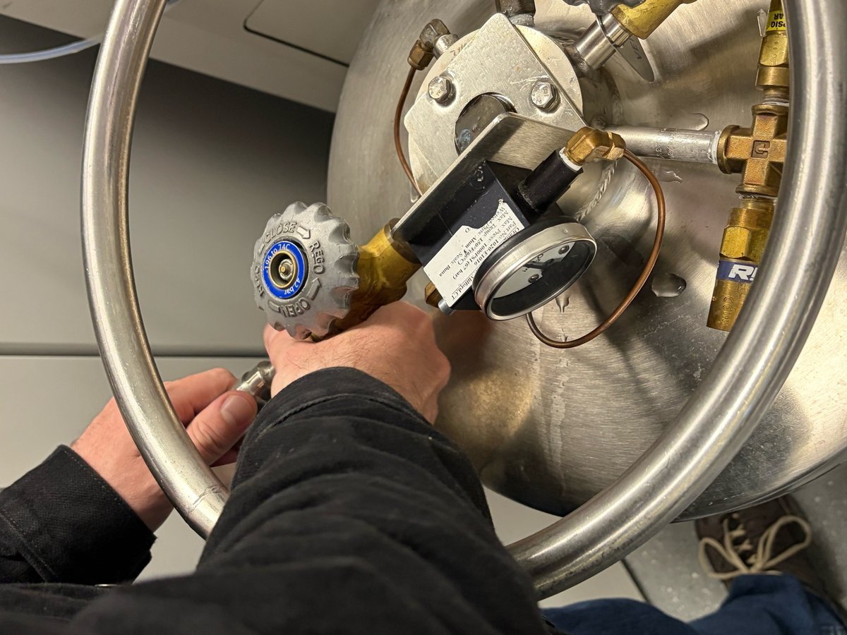
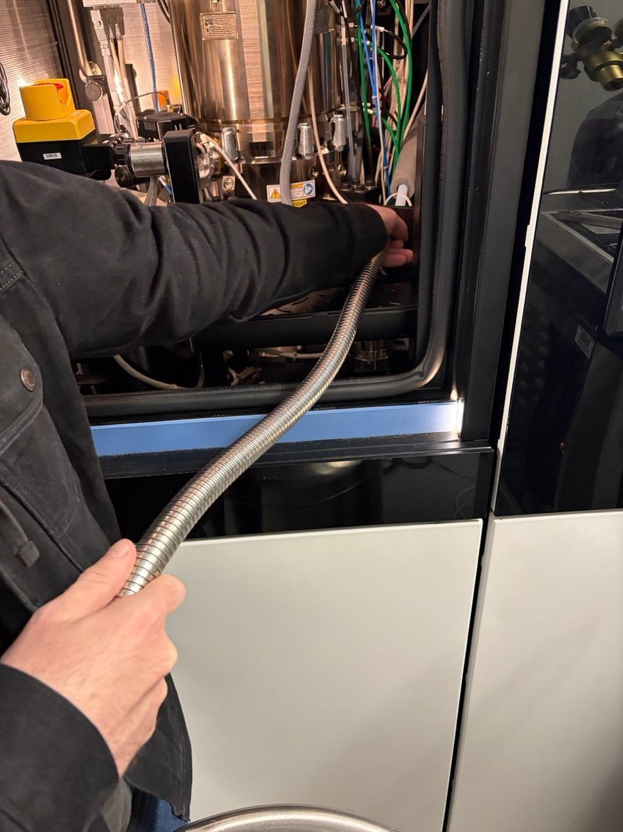
-
Insert the other end of the hose into the fill port on the Spectra.
-
-
Open the valve and fill
-
Open the
LIQUIDvalve by turning the knob counter-clockwise (towardOPEN).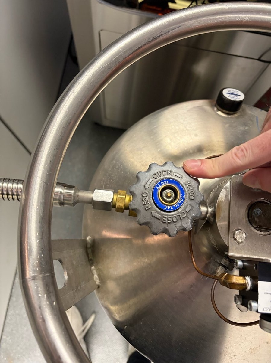
-
Watch the Spectra touch panel
Nitrogen Level. Stop at 80-85% to leave headroom for thermal expansion.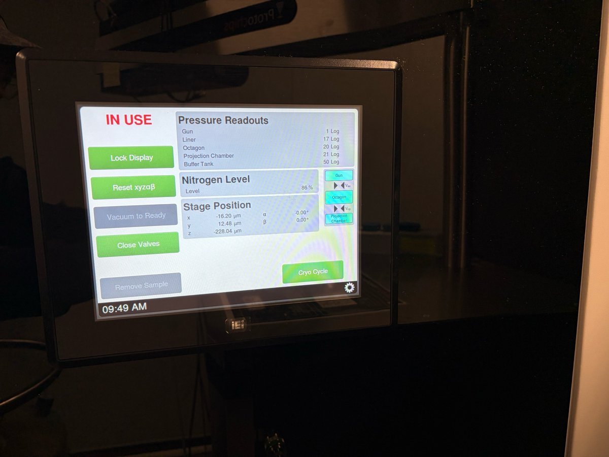
-
-
Close the valve and disconnect
-
Close the
LIQUIDvalve by turning clockwise (towardCLOSE). Use the wrench stored on the dewar handle if the knob is iced over.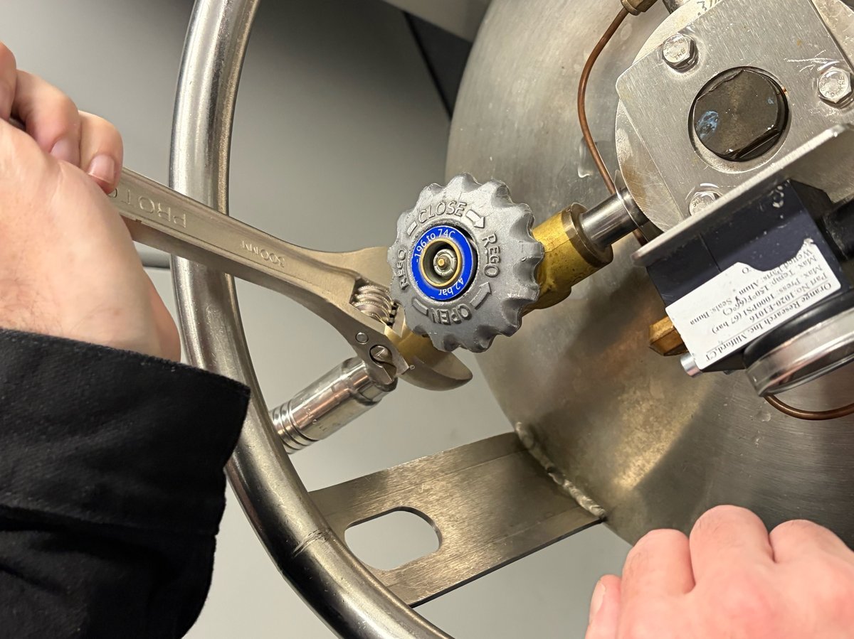
-
Disconnect the hose from the Spectra fill port.
-
-
Return the tank
-
Roll the tank back to the back room. Lock it in place with the safety chain as shown.
-
Octagon recovery
The Octagon vacuum gauge measures the sample-area pressure. If it goes out of range, TEMUI reports an error and the Octagon gauge may show Disabled. Run Evaluate Column and toggle the column ion getter pump (IGPcl) to bring it back.
-
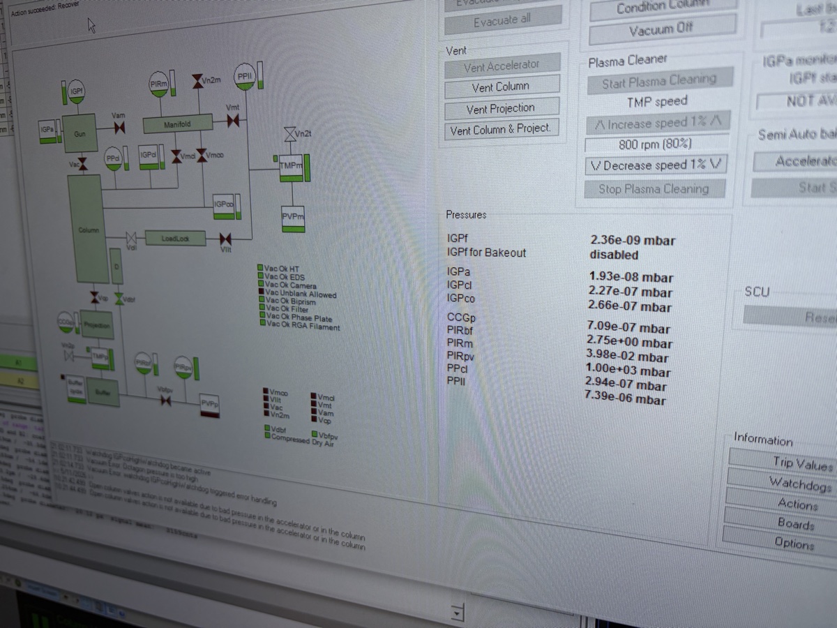
Confirm the Octagon error
-
In
TEMUI, open theVacuum (Supervisor)panel. The Octagon row readsDisabled(or a high log value) when the gauge has tripped.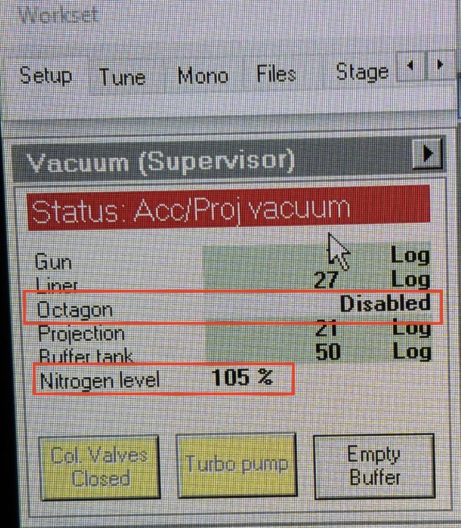
-
Open the error log to read the underlying message. Typical entries include
Vacuum Error: Octagon pressure is too highorWatchdog IGPco High.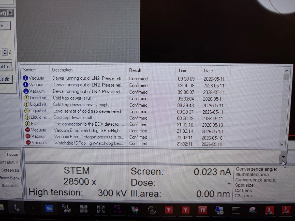
-
-
Run Evaluate Column
-
In
TEMUI, open the vacuum overview and clickEvaluate Column. The status changes toBusyand the action banner readsAction started: Evaluate Column / Waiting for IGP to start.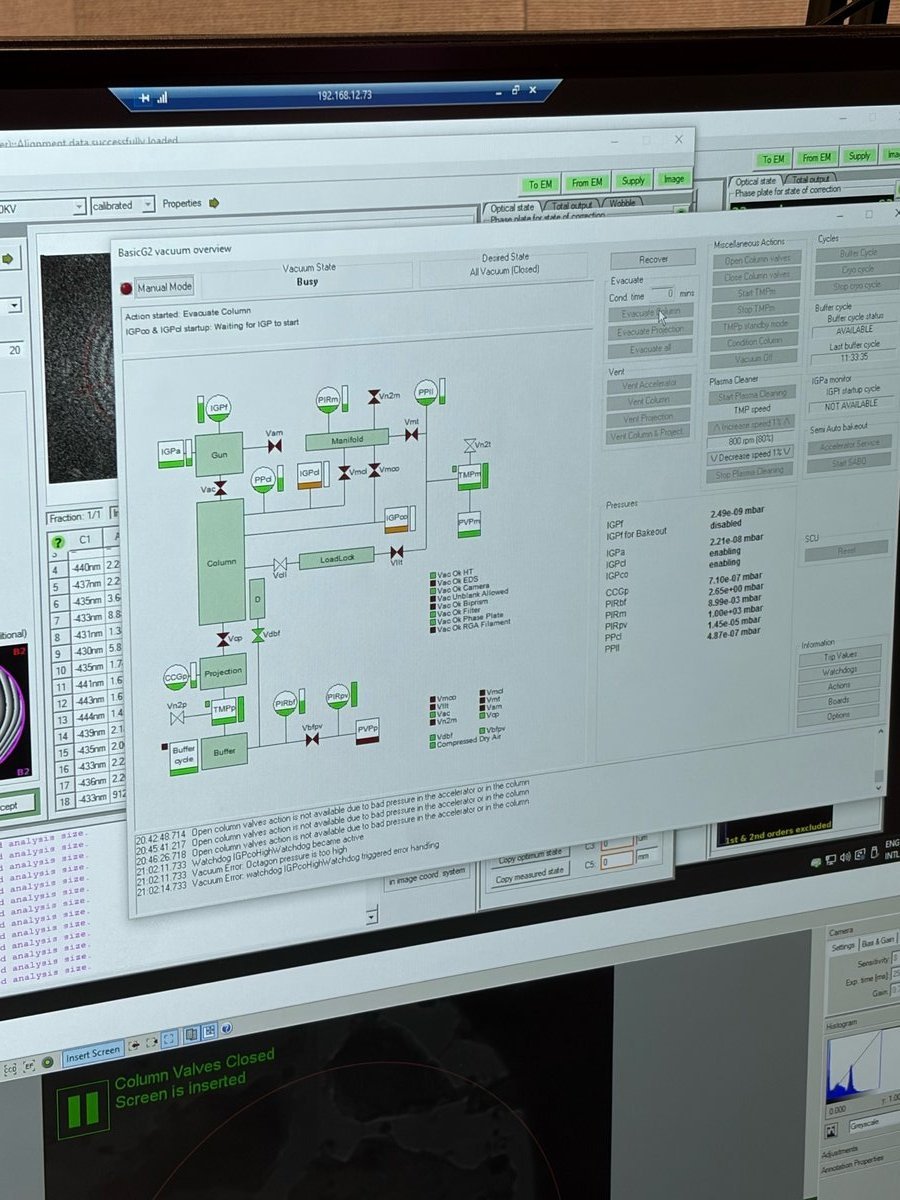
-
-
Toggle the column ion getter pump
-
In the same vacuum overview, click the
IGPclbutton (ion getter pump - column). TheIGPclindicator highlights while the pump cycles.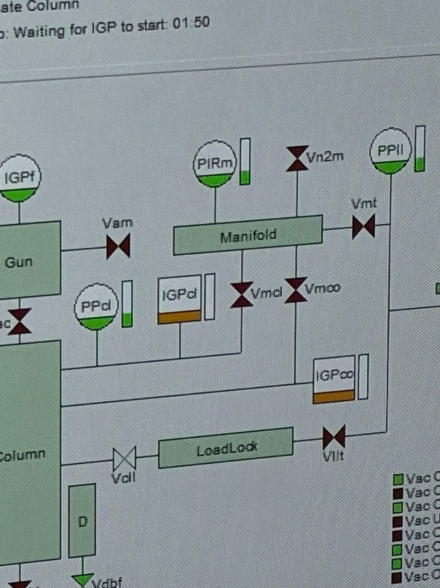
-
-
Wait for recovery
-
Watch the
Vacuum (Supervisor)panel. Status readsBusywhile the system recovers and the Octagon log value drops.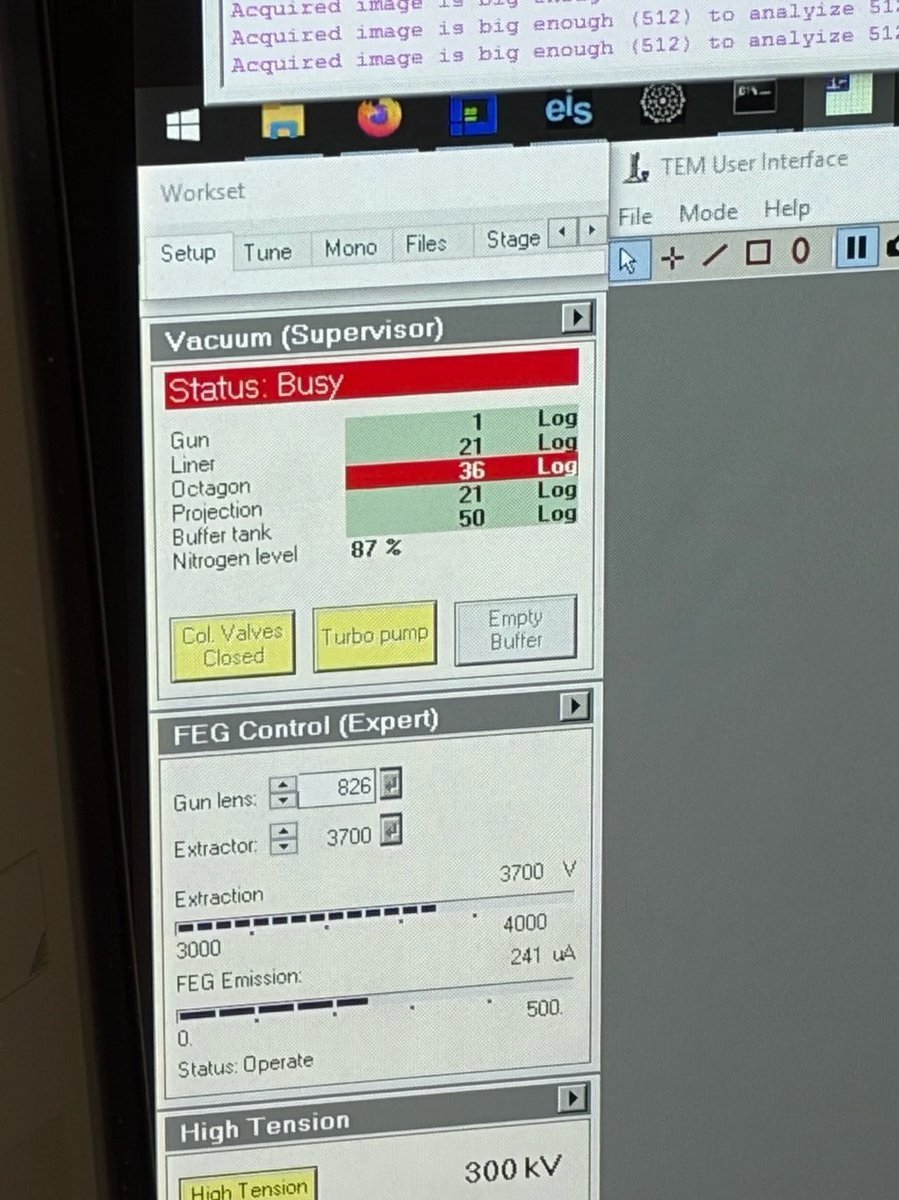
-
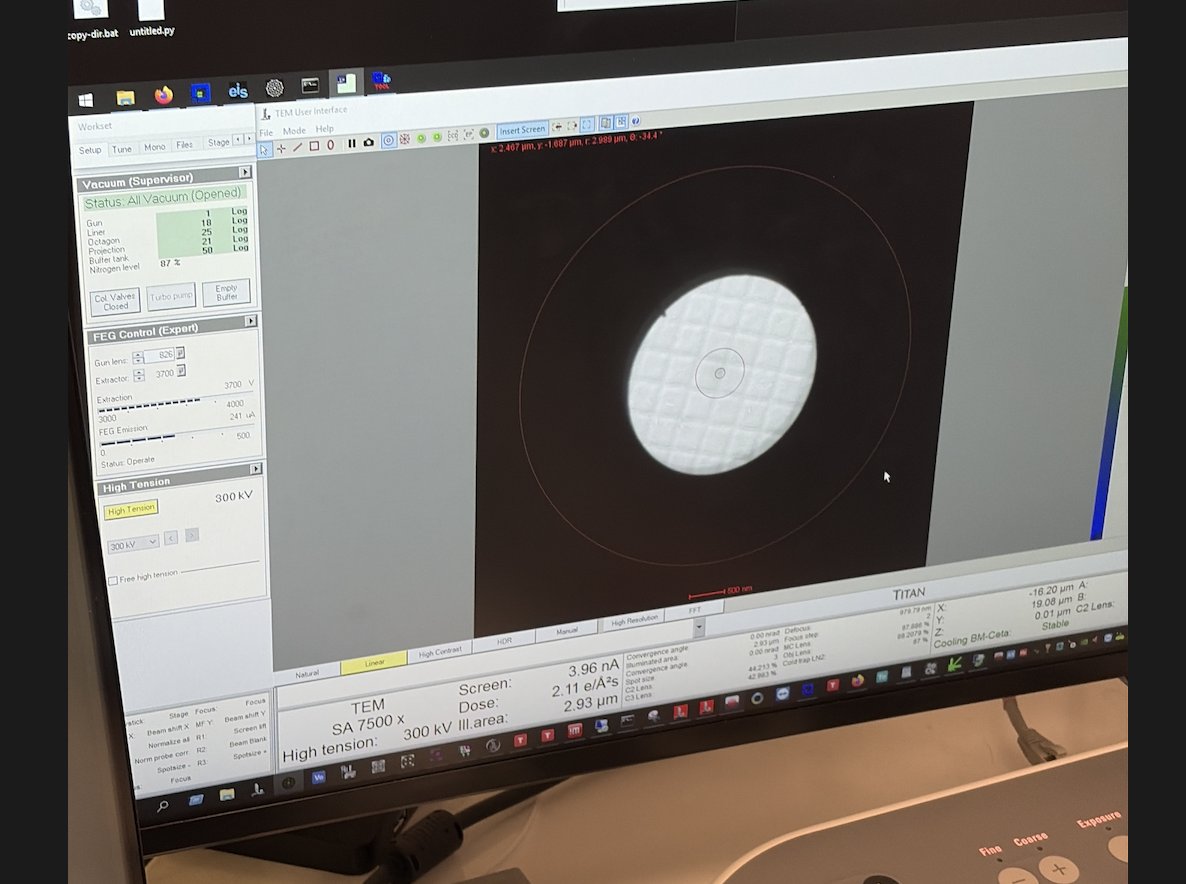
Wait for the Octagon row to return to green. If it does not recover within a few minutes, escalate to staff.
-
Once recovered, return to imaging and verify the beam is visible on the fluorescent screen.
-
Changelog
- May 11, 2026 - Initial draft of Octagon recovery and LN2 fill from staff notes by @bobleesj
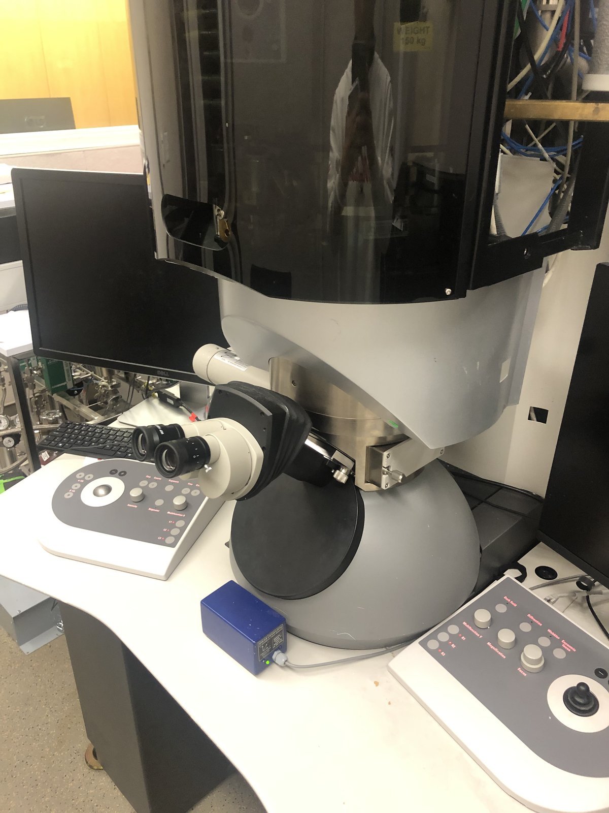
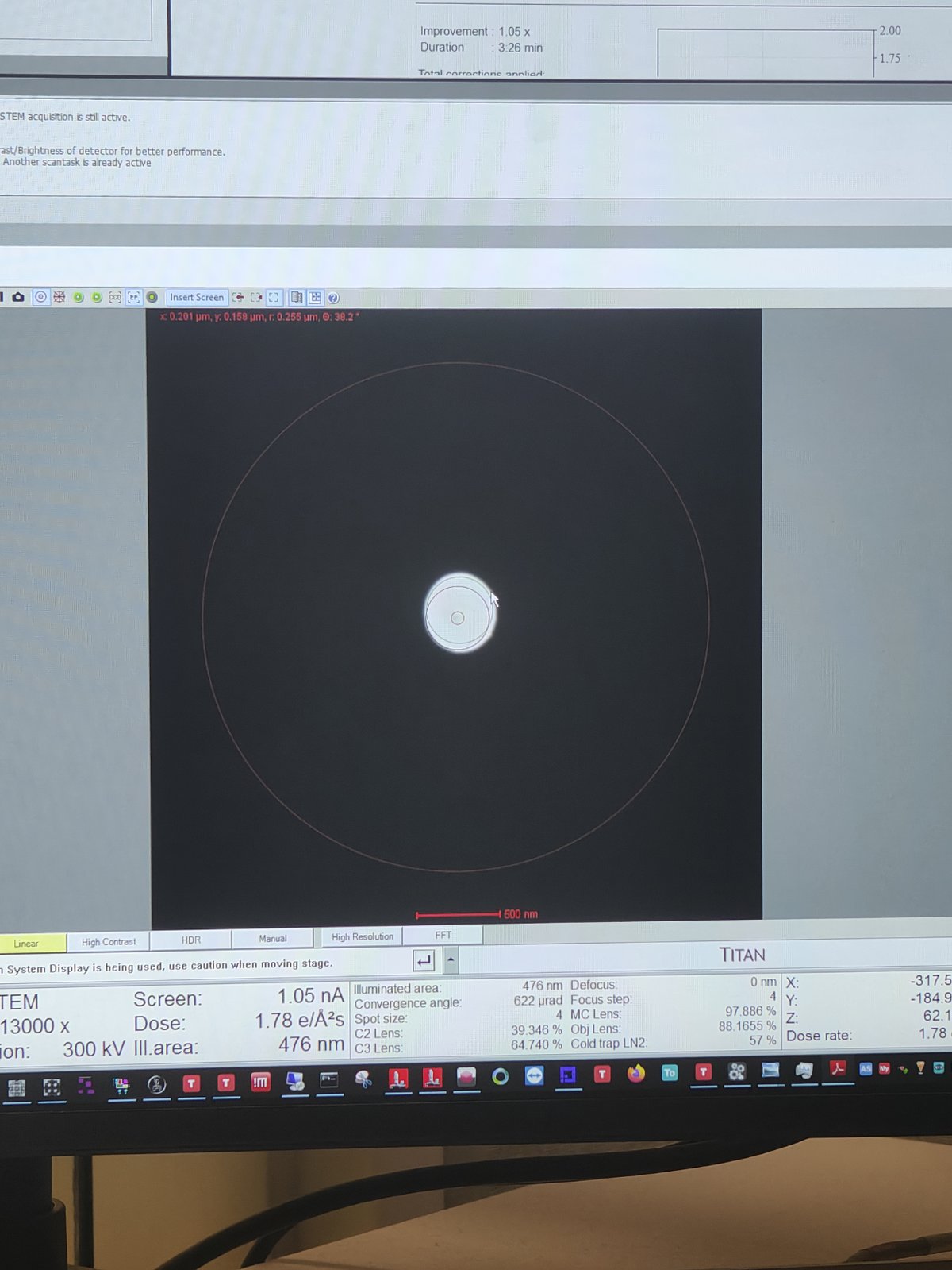
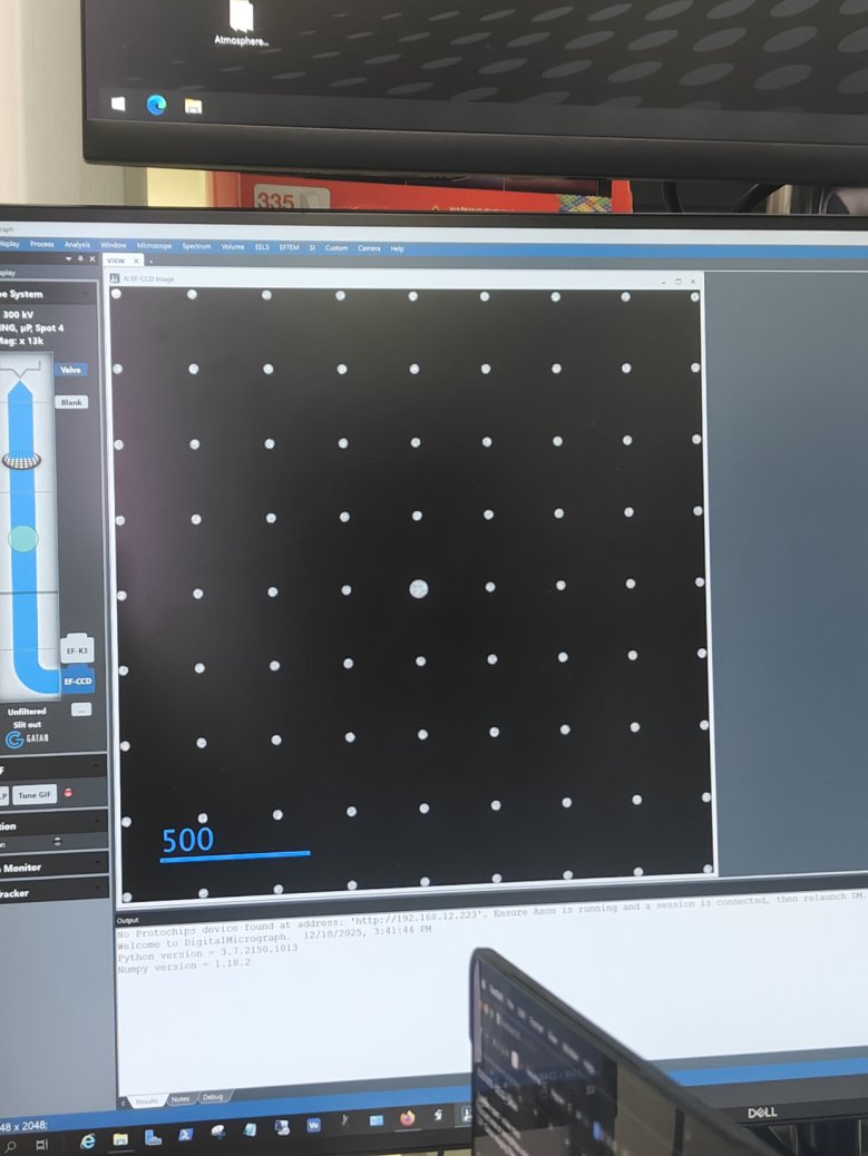
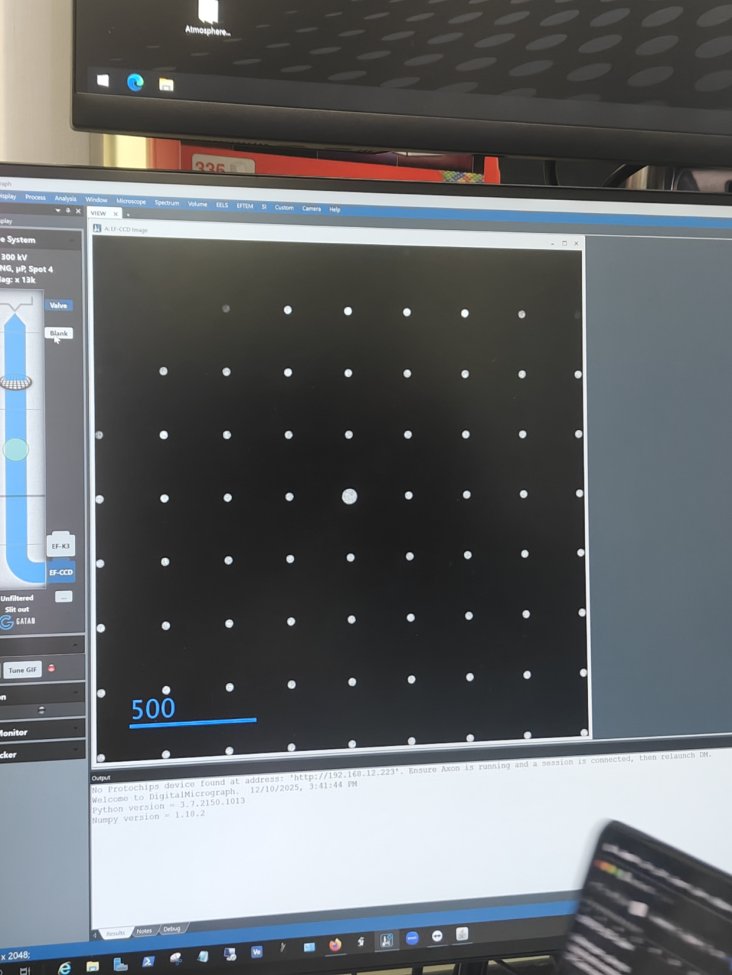
TEM (Titan)
Coming soon.
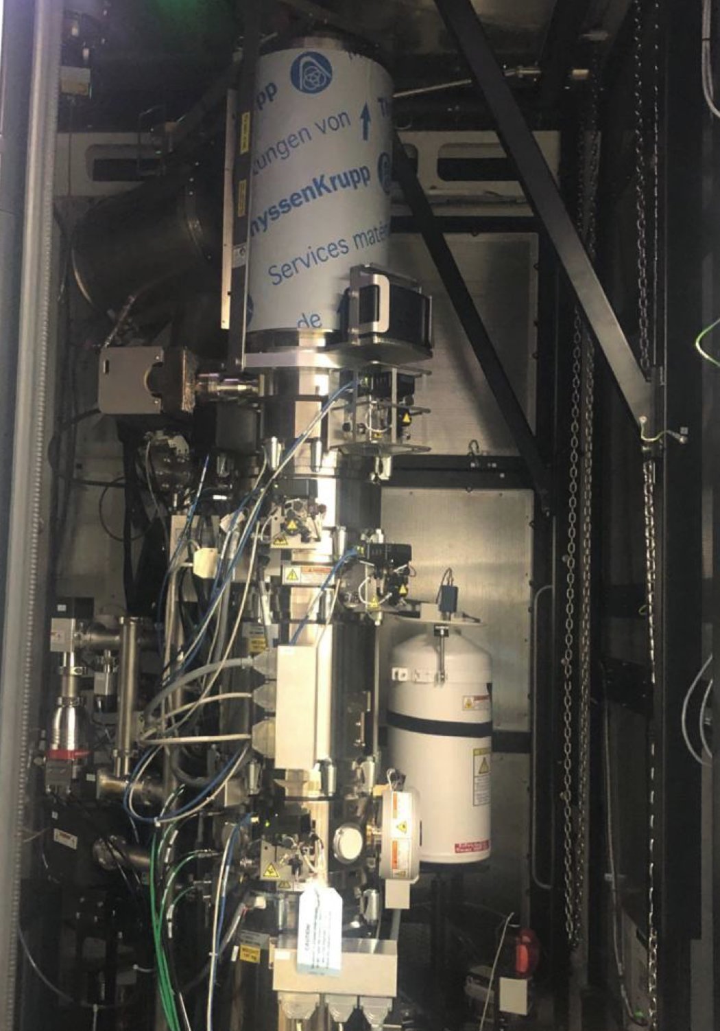
This guide covers TEM alignment and imaging on the FEI Titan at Stanford SNSF.
Changelog
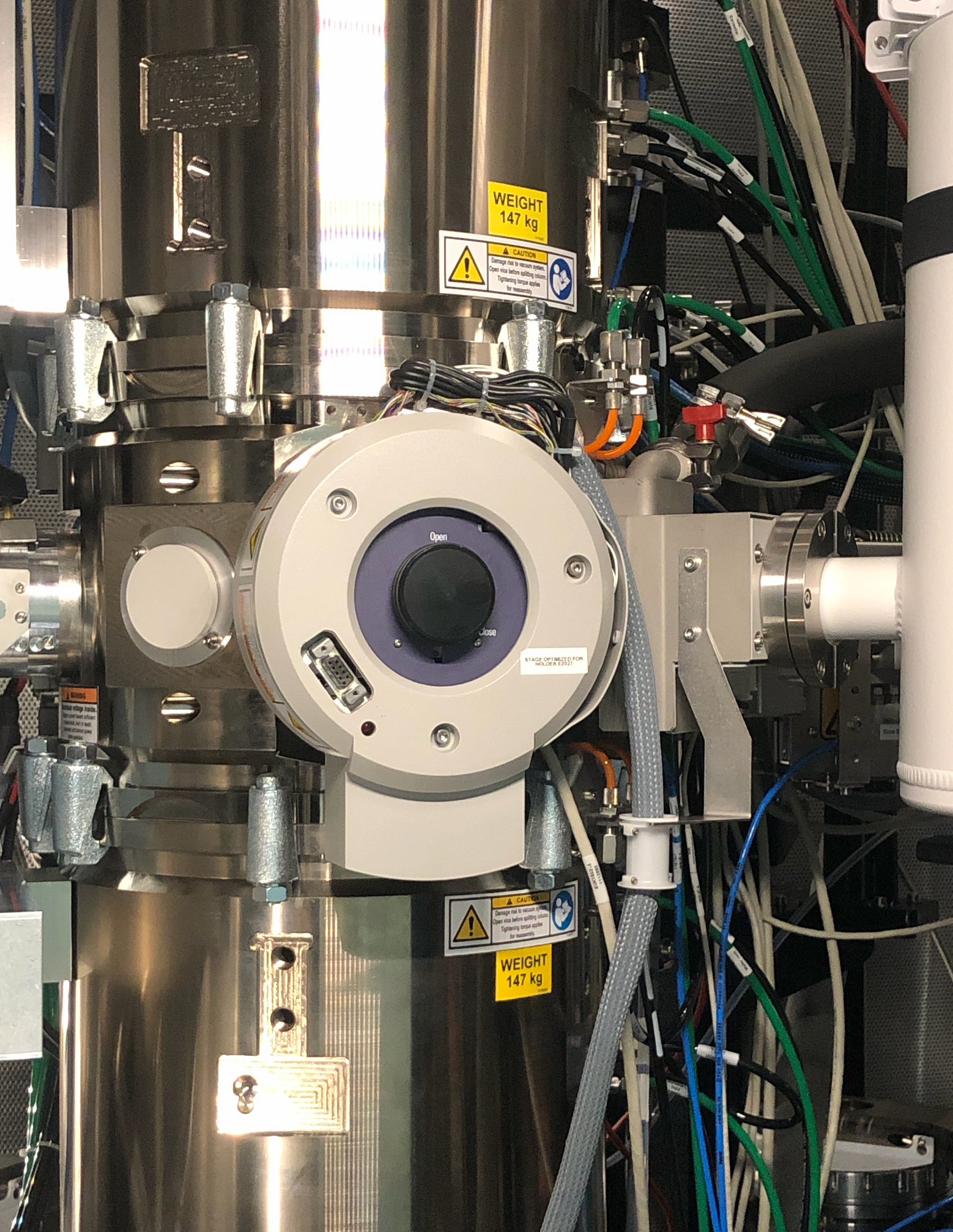
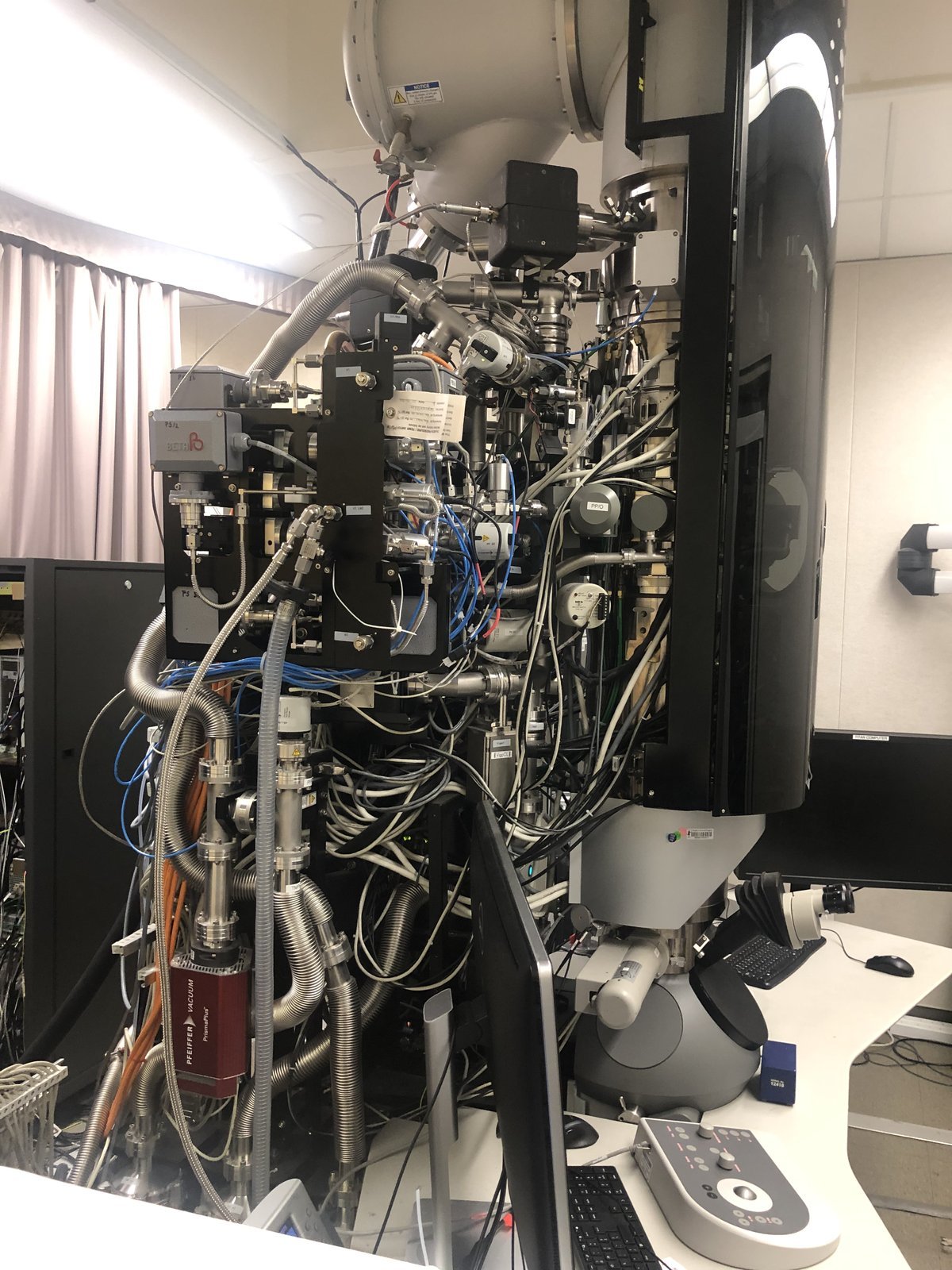
- Feb 28, 2026 - Add Titan instrument photos
4DSTEM
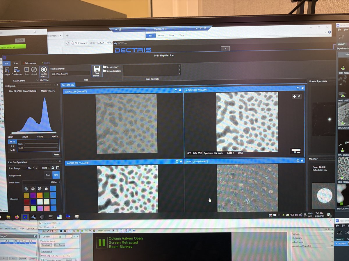
This guide covers 4DSTEM data acquisition using the Dectris Arina detector on the Spectra 300 at Stanford SNSF. 4DSTEM records a full convergent beam electron diffraction (CBED) pattern at every scan position, producing a 4-dimensional dataset (2D scan x 2D diffraction). Screenshots recorded by Guoliang Hu during training; instructions written by Sangjoon Bob Lee.
Prerequisite: Complete TEM (Spectra) column alignment and STEM (Spectra) probe correction before starting this guide.
Acronyms:
mulXY- Multifunction X/Y knobs on hand panelTEMUI- TEM User Interface (software)CBED- Convergent Beam Electron Diffraction
Overview
| Phase | Procedures | Time |
|---|---|---|
| Part 1: Detector setup | Retract CETA, initialize Arina, connect remote software | 5 min |
| Part 2: Beam configuration | Set convergence angle, apertures, camera length (optional) | 5 min |
| Part 3: Acquisition | Insert detector, acquire diffraction data | varies |
| Part 4: End session | Retract and power off the Arina detector | 2 min |
Part 1: Detector setup
1.1 Retract CETA detector
Before inserting the Arina detector, a user must retract the CETA camera. Both detectors occupy the same physical space below the column. If the CETA is not retracted, inserting the Arina will crash both detectors. Do not skip this step.
-
On the bottom left computer, open the blanker/shutter software (red square icon with white T).
-
Click the CETA icon to retract the CETA detector.
-
Visually verify the CETA camera position is retracted from the diagram.
-
In
TEMUI, locate theSTEM Detector (User)panel and verify all detectors are retracted:- HAADF: Retracted
- BF-S (Bright Field): Retracted
- DF-S (Dark Field): Retracted
1.2 Initialize the Arina detector
-
Open the instrument enclosure on the Spectra 300.
-
Locate the Dectris Arina detector unit inside the enclosure.
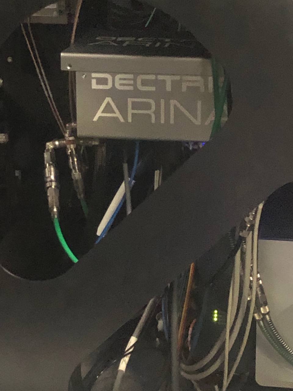
-
Press and hold the button below the Arina detector (blue indicator light) for 10 seconds. When powered on, the button stays pressed in and the blue light is illuminated.
1.3 Connect remote software
-
On the control workstation, open Firefox and click the remote connection bookmark.

-
Enter the detector IP address:
192.168.12.73. -
Click
Initialize detector. Wait for initialization to complete before proceeding. The interface shows a progress bar while the detector initializes.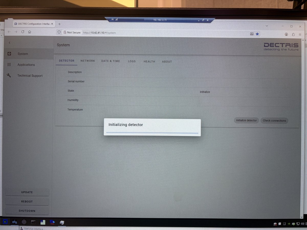
1.4 Configure file saving
-
Open the NOVENA detector software.
-
Click
Save Imagesand select the destination folder.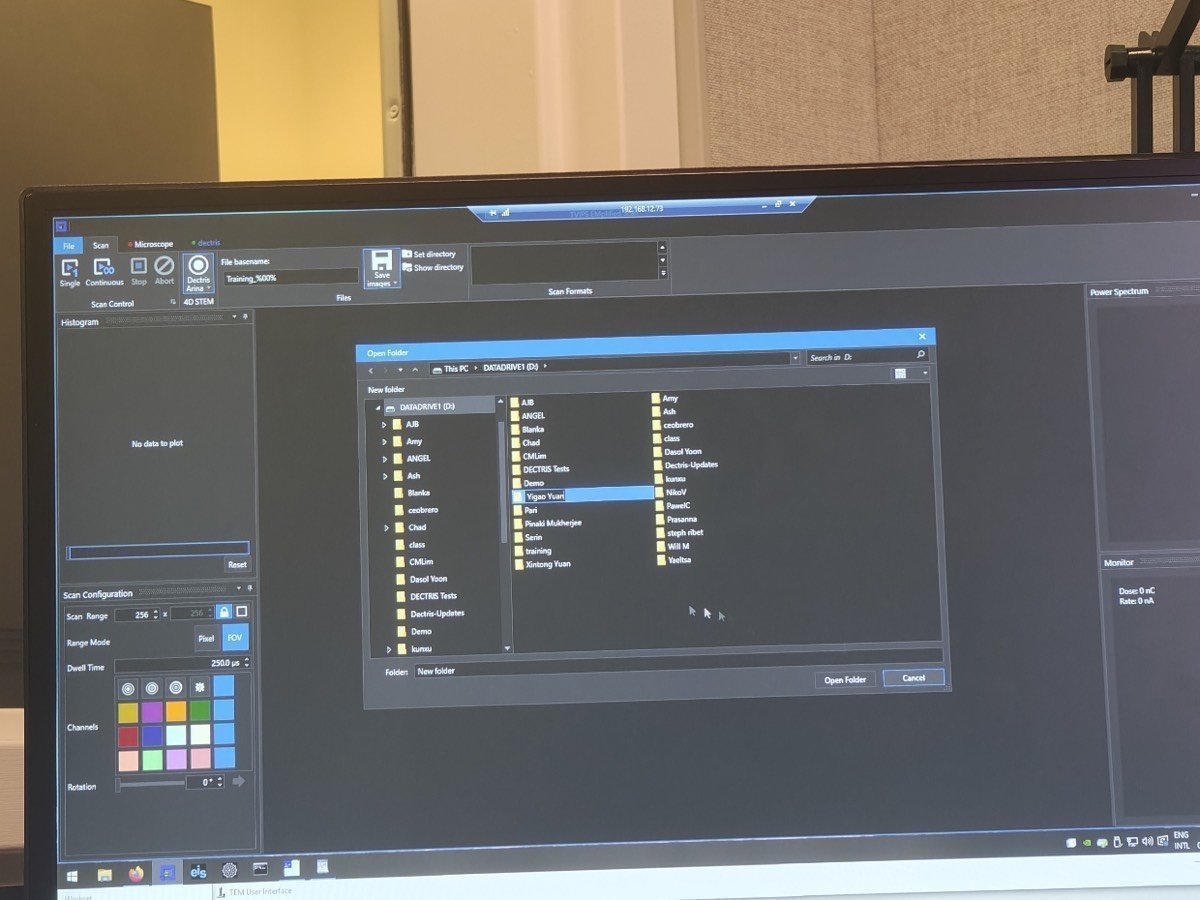
-
Set the filename format to
(name)_%00%. The%00%placeholder auto-increments the frame number. -
Use
Continuousfor live streaming (preview) andSingleto record and save a dataset.
Folder and file naming convention
A consistent naming convention saves hours of searching later when sharing data or revisiting a session months later. Use the patterns below.
Use lowercase everywhere: folder names, sample names, operator names, all tokens. Lowercase removes the question of whether a file should be
GoldorgoldorGOLD, keeps shell paths simple, and sorts cleanly.
Folder name: YYYYMMDD_{sample}_{experiment}[_{operators}]
Lead with the most important keywords: the sample first, then the experiment or focus. Adding the operators (initials or short names) at the end is optional but highly recommended: it captures who was in the room so the surrounding context (conversations, troubleshooting, follow-up questions) is easier to remember months later.
| Example | Meaning |
|---|---|
20260428_gold_drift_ptycho | Gold sample, drift study via ptychography on Apr 28, 2026 |
20260428_gold_drift_ptycho_dasol_corrie | Same session, with Dasol and Corrie noted |
20260512_mos2_ptycho_bob | MoS₂ sample, ptychography, solo session by Bob on May 12 |
File name: {voltage}_{convergence}_{scan-params}_{notes}.h5 (or .mat, .raw)
Order tokens from the largest concept (session-wide) to the smallest concept (per-scan). Voltage applies to the whole session, then convergence and camera length apply per-experiment, and scan dimensions and dwell time change per scan. Reading the filename left-to-right then reads like zooming in from the broadest setting to the most specific.
| Token | Meaning | Example | Scope |
|---|---|---|---|
{n}kev | Accelerating voltage | 300kev, 120kev | session-wide |
{n}mrad | Convergence angle | 30mrad, 1.5mrad | per-experiment |
cl{n}m | Camera length | cl0.4m, cl1.05m | per-experiment |
{n}x{n} | Scan dimensions | 128x128, 512x512 | per-scan |
{n}us | Dwell time (usually µs on Arina) | 5us, 200us | per-scan |
Only encode parameters that are constant for the whole scan. Skip things that drift or change over time (e.g., defocus): they are not informative as a fixed filename token, and there is no need to record them in the h5 metadata either.
| Example | Meaning |
|---|---|
300kev_30mrad_128x128_5us | 300 kV, 30 mrad probe, 128 by 128 scan, 5 µs per pixel |
300kev_1.5mrad_64x64_nbed | 300 kV, nanobeam diffraction at 1.5 mrad |
300kev_30mrad_256x256_drift1 | First scan in a drift series |
Stick to these patterns from the start of every session so the names sort cleanly in the file browser and stay searchable.
Part 2: Beam configuration (optional)
The STEM (Spectra) guide sets 30 mrad convergence angle by default. If that is suitable for your experiment (e.g., ptychography), skip this section and go directly to Part 3: Acquisition. If you need a different convergence angle (e.g., nanobeam diffraction), follow the steps below.
Why change the convergence angle for 4DSTEM?
The convergence angle depends on the type of 4DSTEM experiment. For ptychography, 30 mrad (the same as standard STEM) works well because overlapping disks are part of the reconstruction. For nanobeam diffraction, where separated Bragg disks are needed to index reflections, a much smaller angle is used, typically 1 to 10 mrad depending on the material and the required disk separation.
Interactive demo: Explore how convergence angle affects the CBED pattern at bobleesj.github.io/electron-microscopy-website/cbed
2.1 Enable descan
- In
TEMUI, locate theSTEM Imaging (Expert)panel and enableDescan.
2.2 Configure beam for nanobeam diffraction
The default STEM setup uses C2 = 70 and 30 mrad convergence angle. For nanobeam diffraction, reduce both to get separated Bragg disks. The table below shows typical values:
| Parameter | STEM default | Nanobeam diffraction |
|---|---|---|
| C2 aperture | 70 | 50 |
| C3 aperture | 1000 | 30 |
| Convergence angle | 30 mrad | ~10 mrad |
| Beam current | ~0.150 nA | ~0.032 nA |
| Camera length | 91 mm | 230 mm |
Why change the C2 aperture?
The C2 aperture limits the angular range of electrons entering the probe-forming optics. A smaller aperture (50 vs 70) blocks more off-axis electrons, producing a more coherent beam with cleaner diffraction patterns at each probe position. The C2 aperture size and convergence angle are proportional (approximately 7:1 ratio, e.g. C2 = 70 gives ~10 mrad).
TODO: Confirm the C2 aperture to convergence angle ratio with staff
-
In
TEMUI, go toTunetab, thenApertures. Change C2 from 70 to 50, and C3 from 1000 to 30.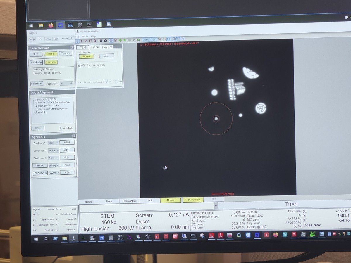
-
In
Beam Setting, clickMF-Y Convergence Angle. Use themulYknob to adjust the convergence angle to 10 mrad, then clickMF-Y Convergence Angleagain to deselect.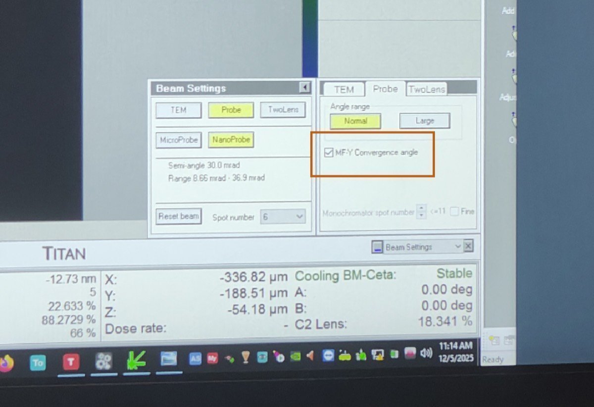
-
Adjust beam current: in
TEMUI, go toMono, clickFocus, and use the intensity knob to set the current to ~0.032 nA. -
Set the camera length to 230 mm (or 285 mm depending on the required angular range for your material).
2.5 Retract HAADF
- In
TEMUI, retract the HAADF detector. The HAADF ring would block electrons from reaching the Arina detector below.
Part 3: Acquisition
3.1 Insert detector and configure scan
-
On the Arina hand panel, press
Insertto move the detector into position. The green “Inserted” light confirms the detector is in place. -
On the scan control box, press
EDS Scan.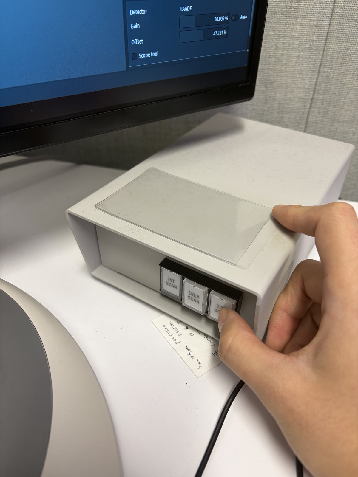
-
Press
R1on the hand panel to lift the fluorescent screen. The Arina detector sits below the screen.
3.2 Acquire data
-
In the NOVENA software, click
Scan, thenContinuousto start a live preview. Verify the central beam is centered on the detector. -
If the beam is off-center, use the
mulXYknobs with diffraction shift to center it. -
Once centered, click
Stop, then clickSingle Scanto acquire and save the dataset. -
After every
Single Scan, verify the dataset was actually saved in the destination folder before starting the next acquisition.NOVENAoccasionally completes a scan without writing the file.-
Confirm both
.h5and_master.h5files are present- Open the destination folder set in Section 1.4 and confirm both files for the latest scan are there.
-
Confirm file sizes are non-zero
- Check the file sizes in the folder. If either file is 0 KB, the save failed and the scan must be re-run.
NOTE: Each scan produces a 4D dataset: a CBED pattern at every pixel in the scan area. File sizes can be large depending on scan resolution and detector binning.
-
3.3 Quick analysis
- In the NOVENA software, use
RebinandReprocessfor a quick check of the acquired data. For detailed analysis, export the data for processing with external software (py4DSTEM, etc.).
3.4 Transfer data to your USB
See how to transfer data to your USB for getting the Arina 4DSTEM datasets and HAADF images off the microscope computers.
Part 4: End session
4.1 Retract the Arina detector
-
On the Arina hand panel, press
Retractto move the detector out of the beam path. The green “Retracted” light confirms the detector is clear.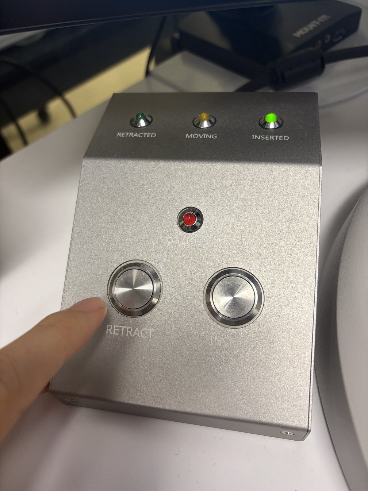
4.2 Power off the detector
- Open the Spectra 300 instrument enclosure.
- Press and hold the button below the Arina detector for 10 seconds. The button releases and the blue indicator light turns off.
4.3 Close session
Follow the steps in End session.
Changelog
- Feb 28, 2026 - Rewrite SOP by Sangjoon Bob Lee with full procedural instructions, inline FAQ dropdowns, and new images
- Dec 10, 2025 - First draft and images shared by Guoliang Hu
EELS
Caution
VERY ROUGH DRAFT - @bobleesj and Guoliang Hu took notes and pictures during training. This document will be updated with more detailed steps and images.
TODO:
- Add image for “EELS Scan” button (Step 2, Part 3)
- Better photo for STEM SI button
- Show what auto gain looks like
- Clarify zero loss extraction steps
- Add comparison images for beam not centered
This guide covers Electron Energy Loss Spectroscopy (EELS) on the Spectra 300. The process has two parts: calibration in TEM mode and STEM EELS spectrum imaging.
Prerequisite: Complete the STEM alignment procedure before starting.
Acronyms:
GIF- Gatan Imaging FilterEFTEM- Energy Filtered Transmission Electron MicroscopyZLP- Zero Loss PeakSI- Spectrum ImagingmulXY- Multifunction X/Y knobs on hand panel
Part 1: Calibration
Use a vacuum or thin amorphous carbon area for calibration.
-
Find a calibration area
- Locate a vacuum region or thin amorphous carbon area on the standard sample
-
Open DigitalMicrograph
-
Open
DigitalMicrographon the left monitor -
If you see any dialog box, click
OKto dismiss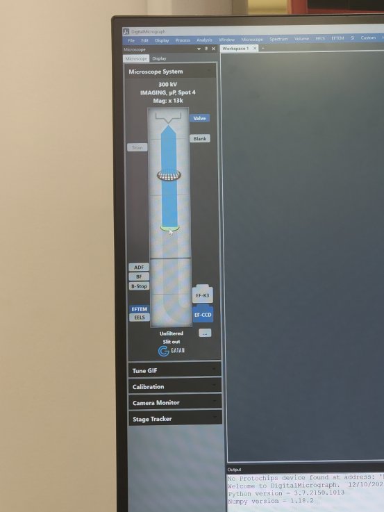
-
Click
EFTEM(Energy Filtered Transmission Electron Microscopy)
-
-
Open FilterControl
-
Go to
Help→User Mode→Power User -
Go to
Window→Floating Window→Filter Control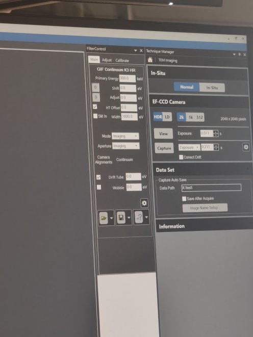
-
Notice the green circle in
TEMUIshowing EELS detector is active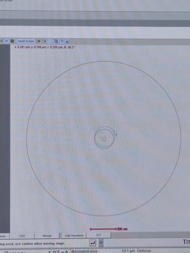
-
-
Set beam intensity
-
Converge the beam by adjusting the intensity knob
-
Lift the fluorescent screen by pressing
R1 -
Click
Viewin DigitalMicrograph -
Go to
Filter Control→Aperture→Maskto verify beam positionCorrect intensity:
Too high intensity (oversaturated):
-
-
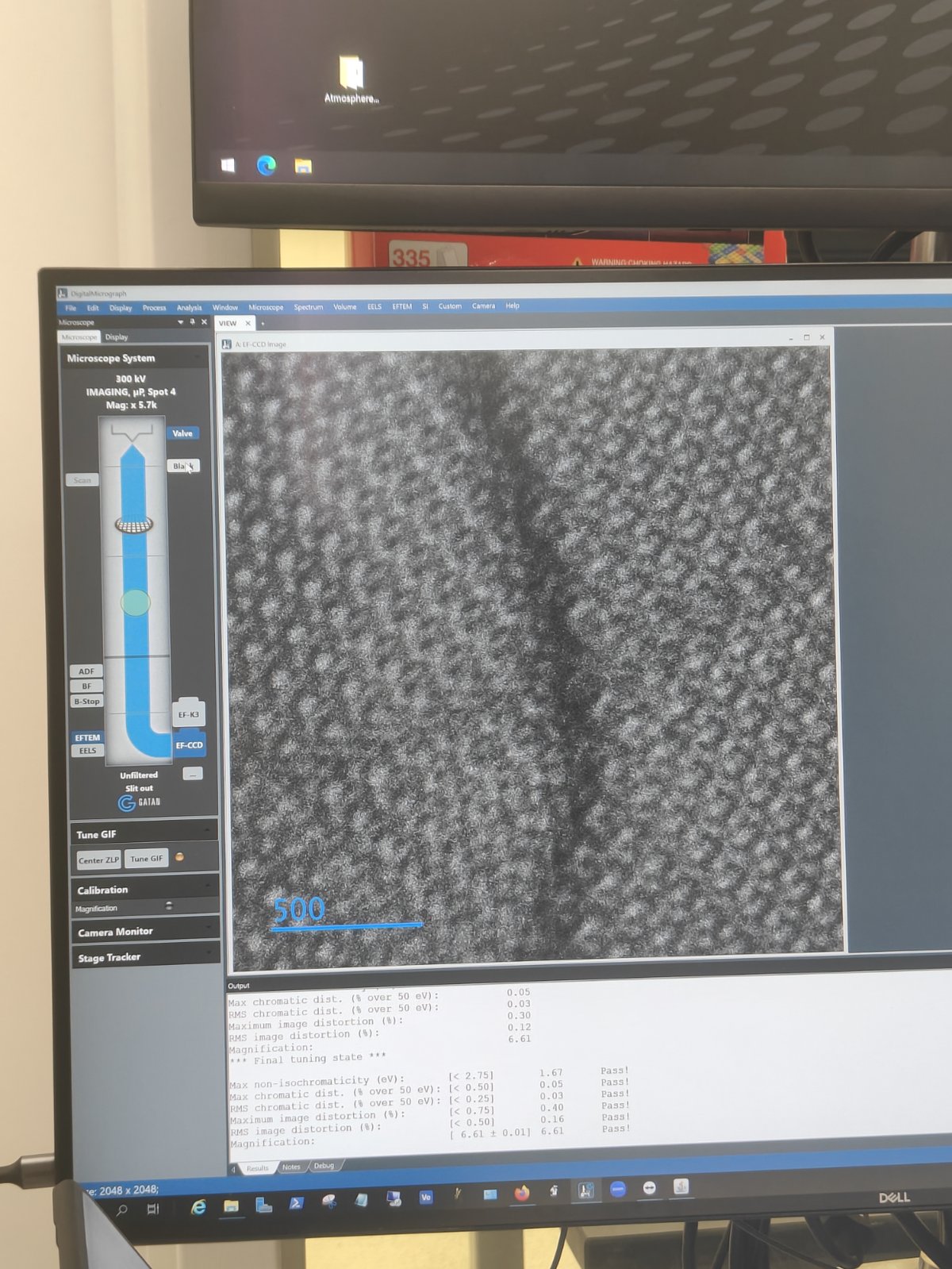
Center and tune the GIF
-
Click
Center ZLPin Filter Control -
Click
Tune GIF. Notice the message appears: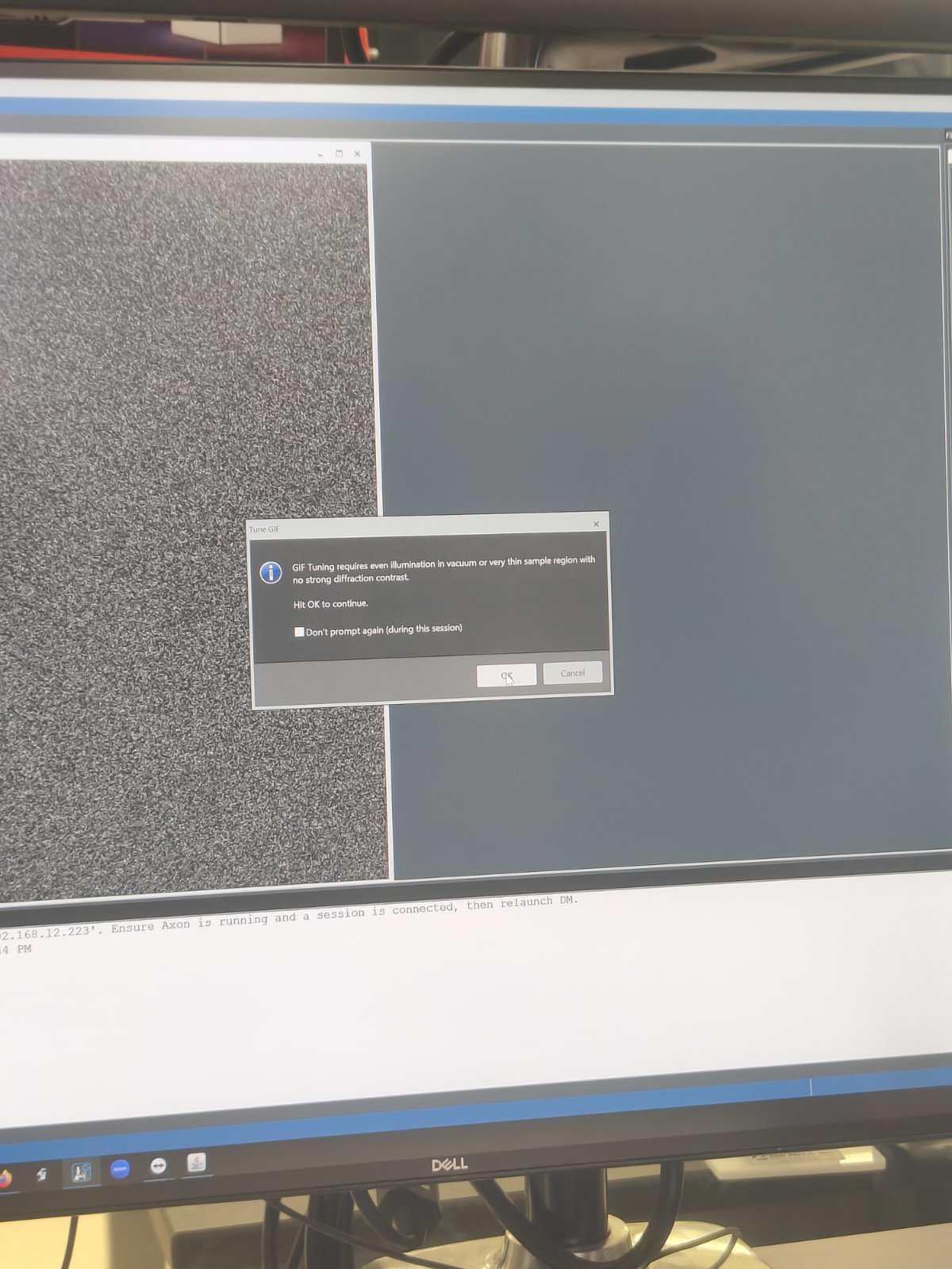
-
Click
OKto confirm
-
Part 2: TEM EELS acquisition
-
View the sample
-
Set magnification to ~17,000x
-
Click
Viewin DigitalMicrograph -
Select
EF-CCD Camera→Viewto see image real-time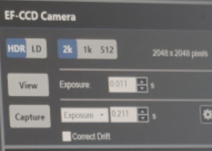
-
-
Acquire zero loss image
-
Go to
SingleMap→ clickZero Loss Image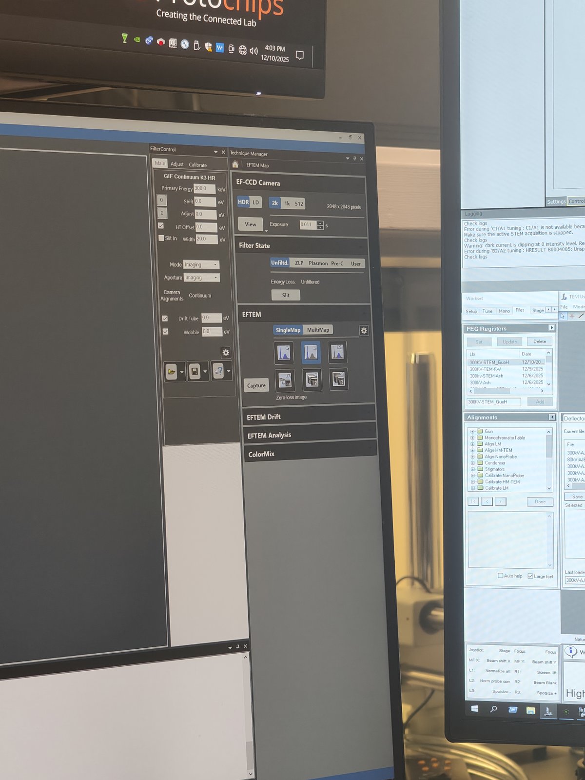
-
-
Switch to EELS mode
-
Click
EELSbutton to switch modes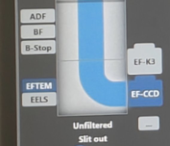
FIXME: use image where EELS is clicked
-
Notice the 2D EELS spectrum. Observe the plasma peak near the zero loss peak.
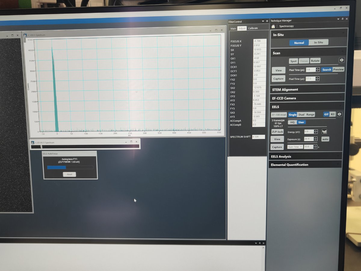
FIXME: what’s plasma peak?
-
-
Align the zero loss peak
-
Set exposure to 2e-4 in View mode
-
Click
Align ZLP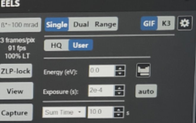
FIXME: where is ZLP click?
-
Part 3: STEM EELS spectrum imaging
-
Set camera length
-
In
Velox, change camera length to 29 mm or 37 mm -
Notice the beam size decreases
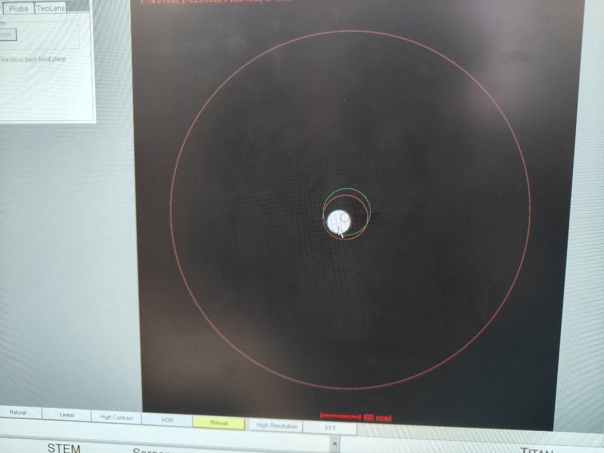
-
-
Enable EELS scanning
- Press
EELS Scanin the software
FIXME: attach image
- Press
-
Find a vacuum area
- Navigate to a vacuum region for initial alignment
-
Center the beam
-
In EFTEM mode, use
mulXYknobs to center the beamBefore centering:
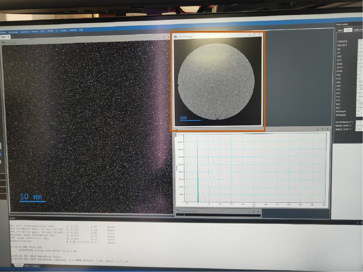
After centering:
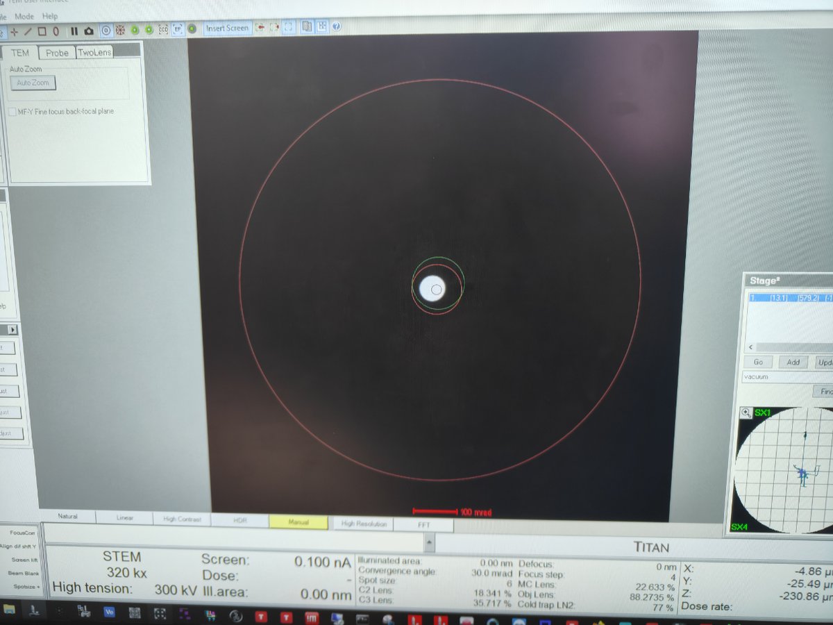
-
-
Switch to STEM SI mode
-
Click
STEM SIto switch to Spectrum Imaging mode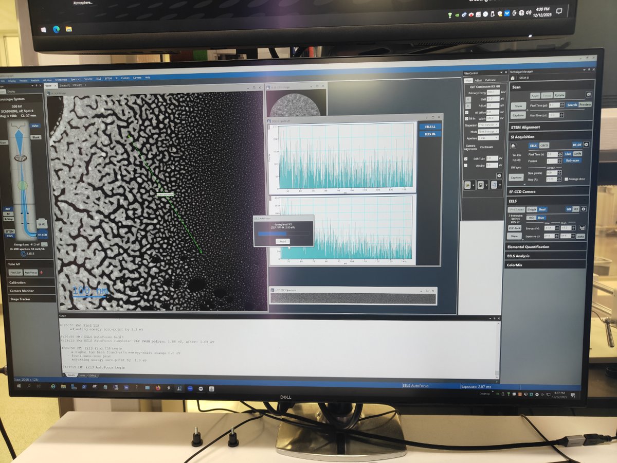
-
-
Find sample area
- Navigate to an area of interest on your sample
-
Start scanning
-
Click
Scan→Viewto see the image
-
-
Adjust gain
- Right-click on ADF image → click
Auto Gain
FIXME: add image showing auto gain result
- Right-click on ADF image → click
-
Stop viewing
- Click
Viewagain to stop live scanning
- Click
-
Capture line scan (1D EELS)
-
Click
Captureand draw a line across the region of interest
-
Go to
EELS→User Mode
-
Go to
EELS→Zero Loss→Extract Zero Loss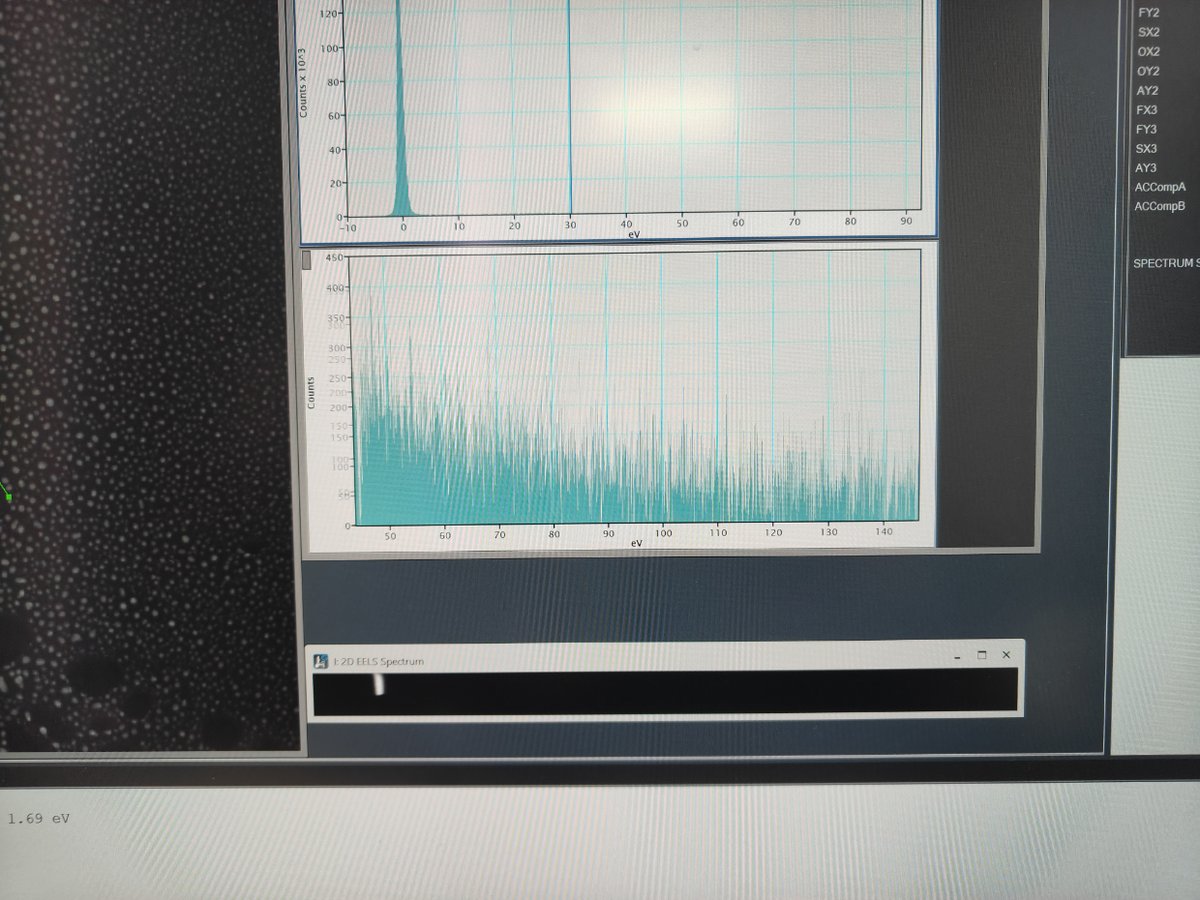
FIXME: clarify what “extract zero loss” does and expected result
-
-
Capture area scan (2D EELS)
-
Click
Captureand select a rectangular area for 2D spectrum imaging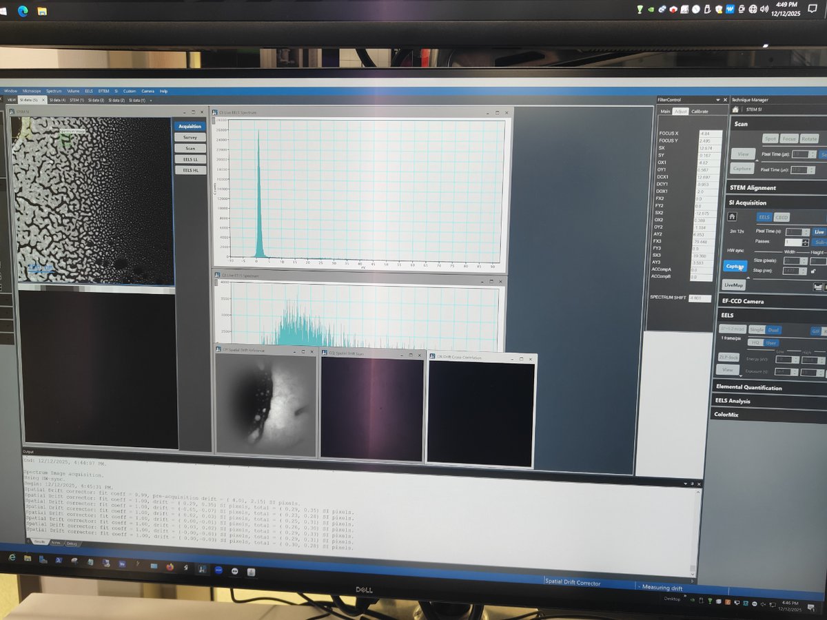
FIXME: add steps for analyzing 2D EELS data, expected output
-
Part 4: End session
Follow the steps in End session.
Changelog
- Dec 18, 2024 - initial rough draft by Guoliang Hu and @bobleesj
EDS
Caution
VERY ROUGH DRAFT - @bobleesj and Guoliang Hu took notes and pictures during training. This document will be updated with more detailed steps and images.
This guide covers Energy Dispersive X-ray Spectroscopy (EDS) on the Spectra 300. EDS identifies elements in a sample by detecting characteristic X-rays emitted when the electron beam knocks out inner-shell electrons. This guide uses the standard gold nanoparticle sample, so Au (gold) is the primary element expected in the elemental maps and spectra.
Prerequisite: Complete the STEM alignment procedure before starting.
Acronyms:
EDS- Energy Dispersive X-ray SpectroscopySI- Spectrum Imaging
Overview
| Phase | Procedures | Time |
|---|---|---|
| Part 1: STEM mode EDS | Set beam parameters, select imaging area, drift correction, acquire and process data | 15-30 min |
Part 1: STEM mode EDS
1.1 Set beam parameters (optional)
-
Adjust convergence angle and beam current
- In
TEMUI, go toBeam Settings, selectProbe, then clickMF-Y - Change convergence angle to approximately 21.5 mrad for EDS. A larger convergence angle focuses more current onto the sample, increasing the X-ray count rate.
- Increase screen current to ~0.4 nA. Higher beam current generates more X-rays but also increases sample damage. To adjust beam current, see Monochromator tune in the STEM guide.
- In
1.2 Select spectrum imaging area
-
Define acquisition area
-
In
Velox, clickSpectrum Imaging Areaas shown below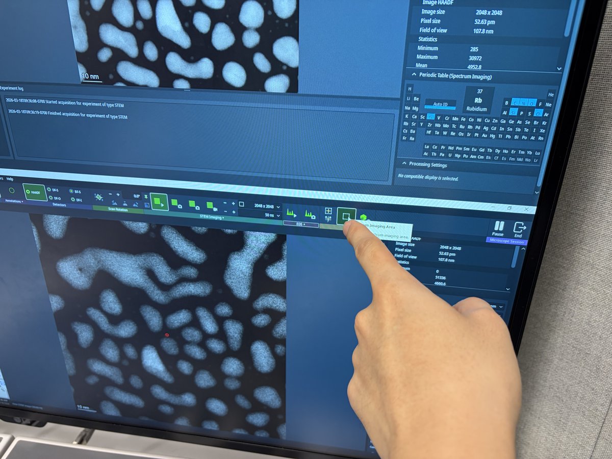
-
Draw a rectangle on the HAADF image to define the area for EDS acquisition
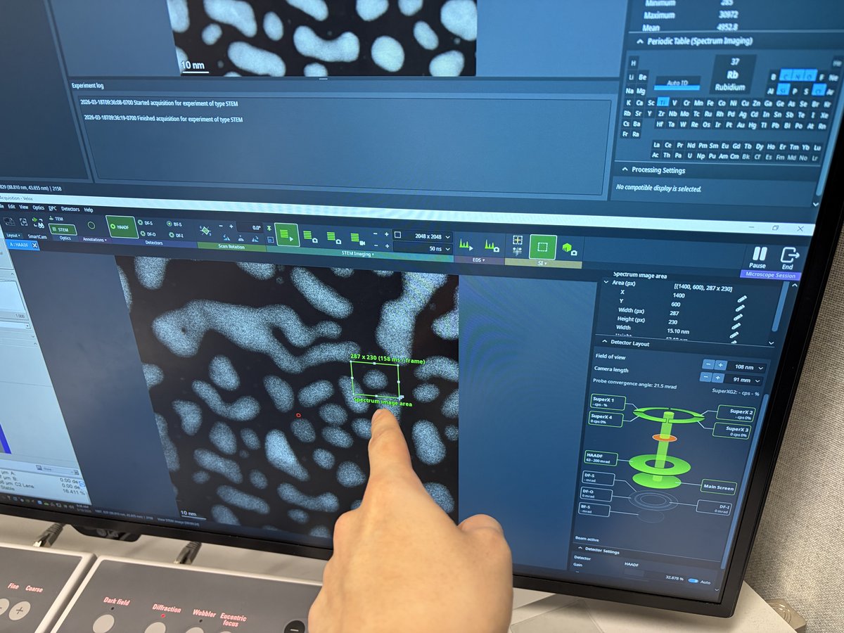
-
-
Set drift correction
-
Click
Drift Areain the toolbar. A tooltip appears: “Draw the drift measurement area.”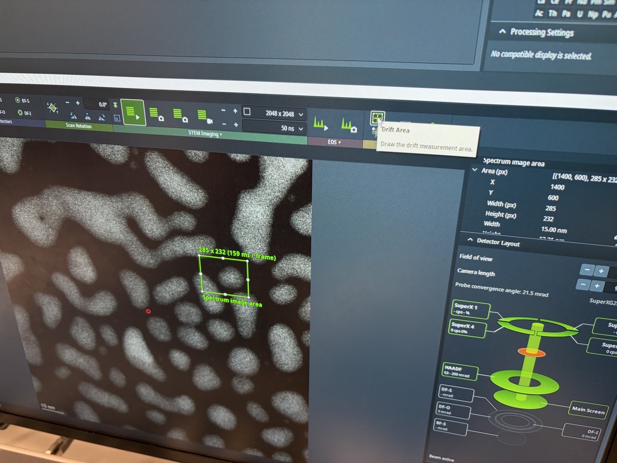
-
Draw a small rectangle near a high-contrast feature. The system uses this region to track and correct specimen drift during acquisition.
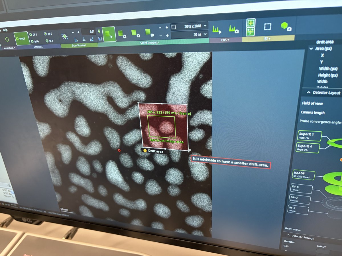
-
Verify both the spectrum image area (green rectangle) and drift area (white rectangle) are visible on the HAADF image.
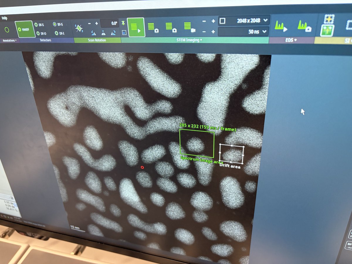
-
1.3 Acquire and process data
-
Start acquisition
-
Click
Spectrum Imagingto start acquisition. The tooltip shows the dwell time per pixel.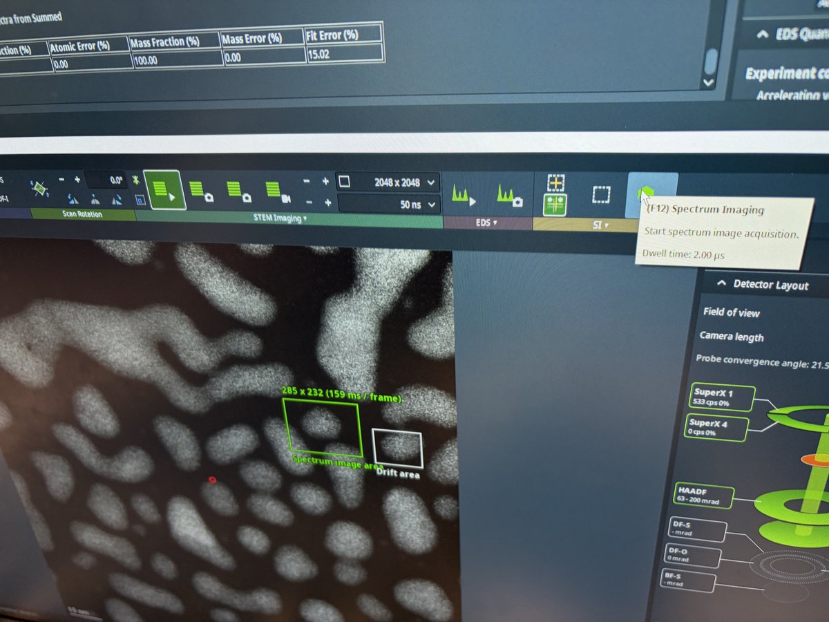
-
Let the acquisition run for several frames so the software accumulates enough signal. Then click
To SpectrumandAuto IDin thePeriodic Tablepanel to identify elements from the spectra collected so far. You may also select elements manually if auto detection does not work.TODO: Verify whether you need both
To SpectrumandAuto ID, or just one of them.
-
-
Review elemental maps
-
Select a rectangular area on the HAADF image for map processing
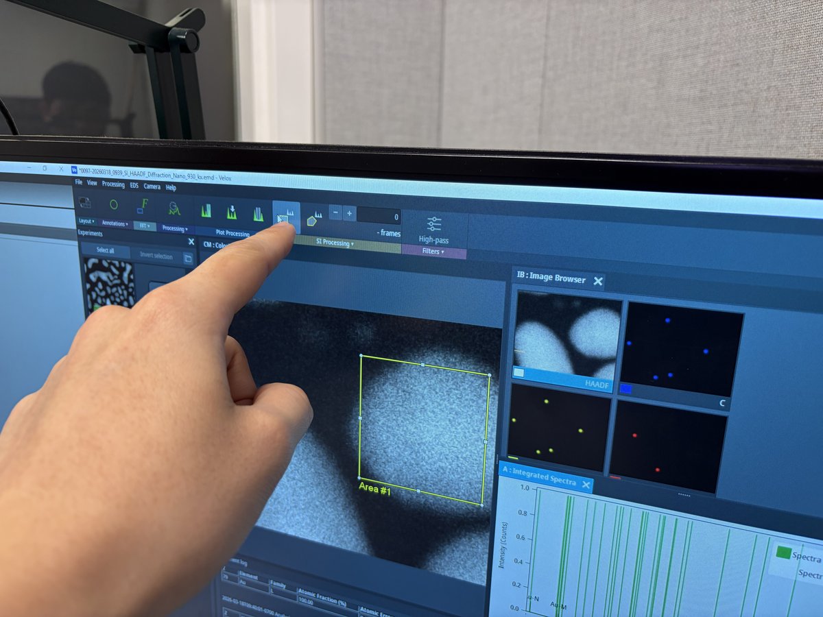
-
The
Image Browserpanel displays elemental maps for each detected element. Use theDisplay Settingson the right to toggle between intensity (int), net counts (net), weight percent (wt%), and atomic percent (at%) views.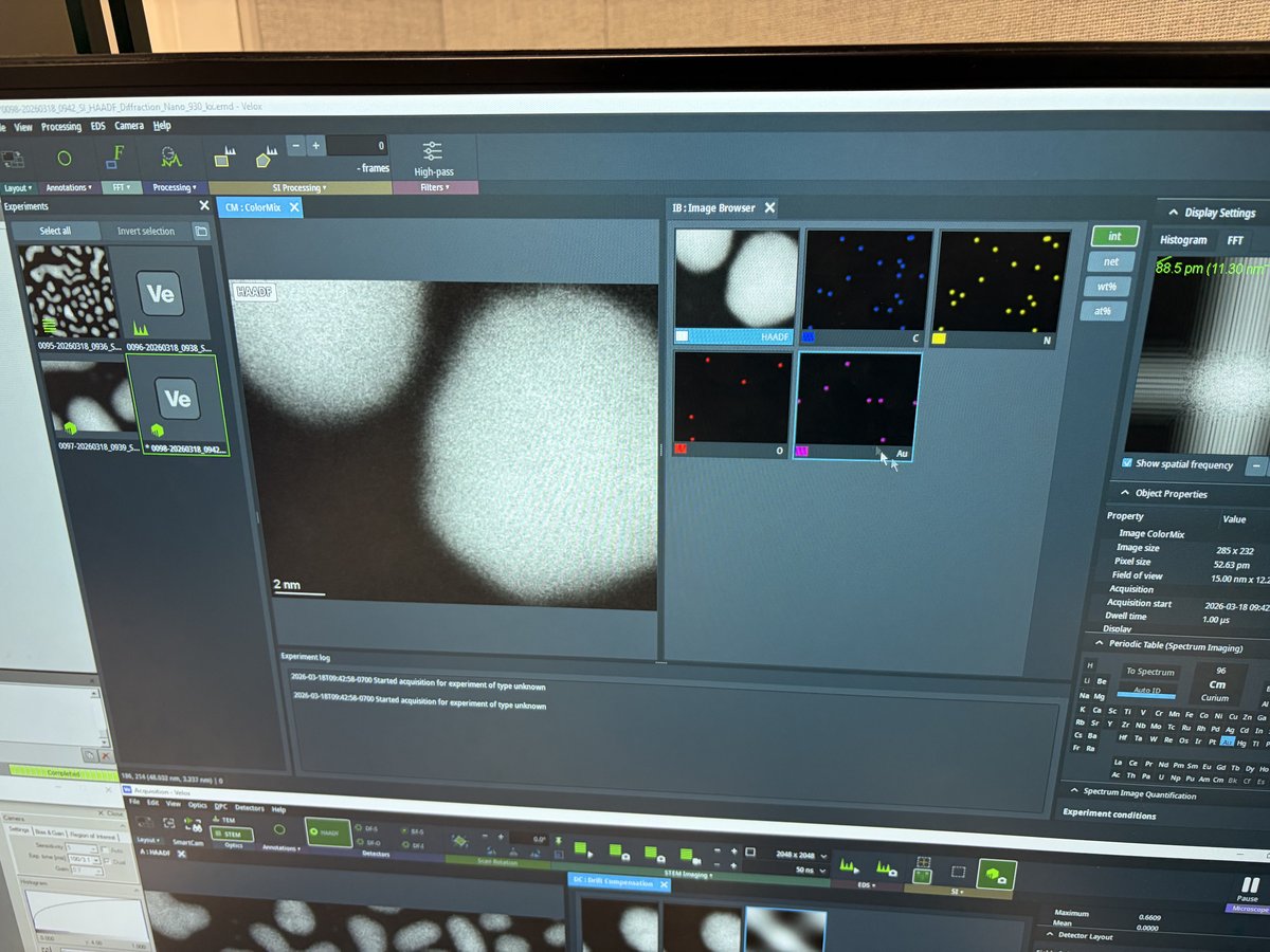
-
The
Integrated Spectrapanel below shows the X-ray spectrum from the selected area. ThePeriodic Tablepanel identifies detected elements. UnderObject Properties, verify the acquisition parameters (image size, pixel size, field of view, dwell time).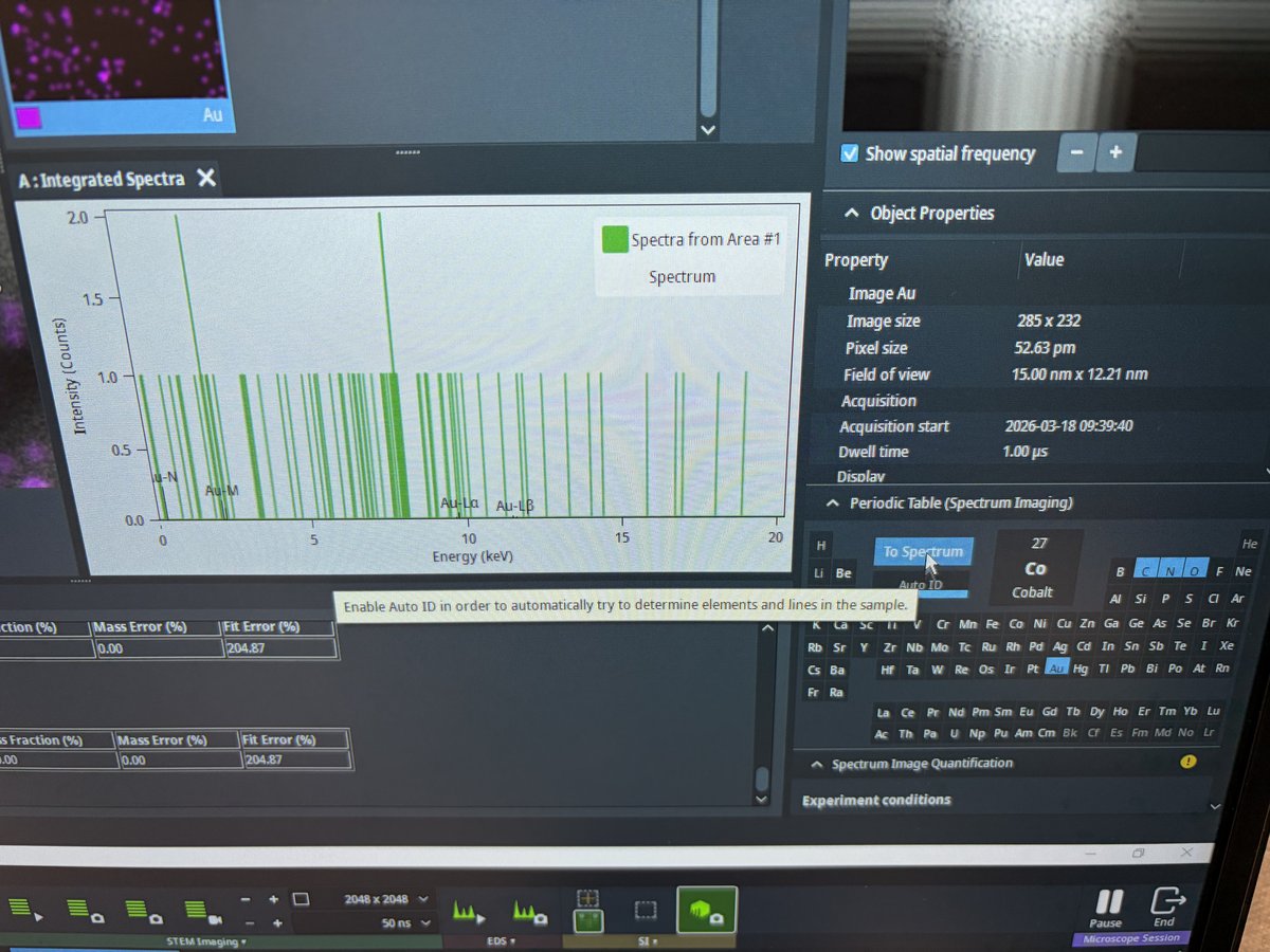
-
Elemental maps show spatial distribution of each element. In this example, N (green/yellow), O (red), and Au (purple) maps are displayed.
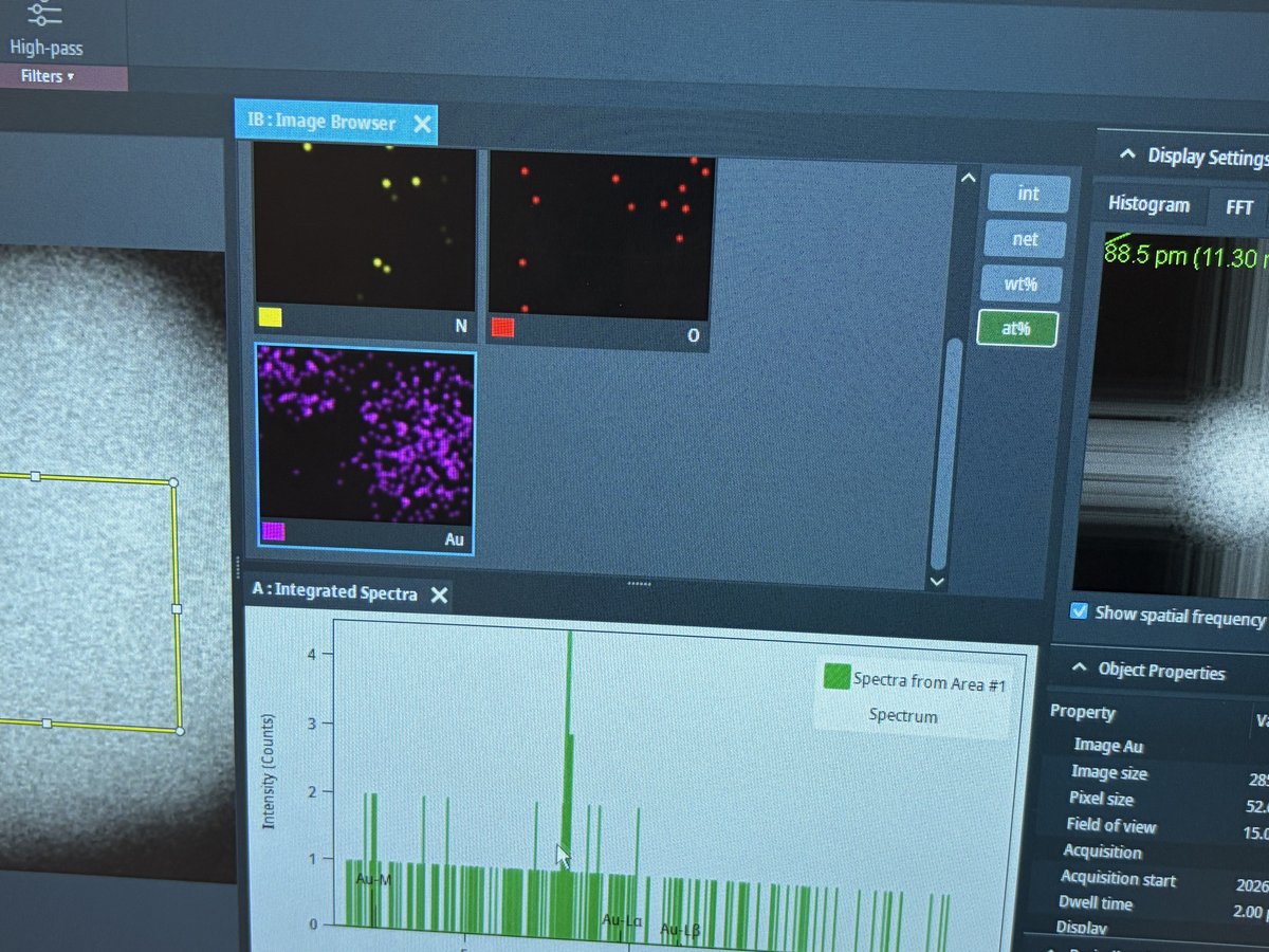
-
End session
Follow the steps in End session from the Spectra STEM guide.
Acknowledgments
Thank you to Cedric Lim for teaching @bobleesj the EDS workflow during his session. Images captured during his session.
Changelog
- Apr 3, 2026 - Replace images with new photos captured by @bobleesj during EDS training by Cedric Lim
- Dec 18, 2025 - Initial rough draft by Guoliang Hu and @bobleesj
Tomography
TODO: Add tomography tutorial content
This guide covers electron tomography on the Spectra 300.
Changelog
- Dec 17, 2025 - Add placeholder by @bobleesj
Ptychography
For the experiment, record the global meta data:
- keV 300 keV
- convergence angle
- spot size
For region of interest, record the following
- Defocus (nm)
- Mag (Mx)
- Scan steps
- dwell time (μm)
- Camera length
- Data collection notes
- Mono
- Current on flucam: 75 pA
- Note (interesting shape? zone axis?)
Random notes:
- Why is it hard to find zone axis in nanoparticles? Small particles (1 - 10 nm)
PED
TODO: Add PED tutorial content
This guide covers Precession Electron Diffraction (PED) on the Spectra 300.
Changelog
- Dec 17, 2025 - Add placeholder
Data transfer: Arina and Velox
This page covers how to get your data off the Spectra computers at Stanford SNSF: Arina 4DSTEM datasets and Velox HAADF .emd images to a USB drive, plus how to mount the lab Mallard network share for remote access. Drafted by Sangjoon Bob Lee from staff notes and images.
Overview
| Task | How |
|---|---|
| Save Arina 4DSTEM data to USB | Plug USB into the Arina PC, copy the dataset |
| Save HAADF images to USB | Copy Velox CaptureData folder to USB |
| Mount the Mallard network share | Map the lab share as a network drive |
Save Arina 4DSTEM data to USB
-
Plug your USB into the Arina PC
-
Plug your USB drive into the computer below (the TVIPS scan generator PC). The USB port is circled.
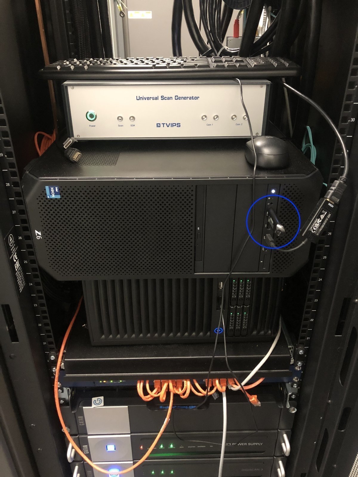
-
-
Copy your dataset to USB
- Open the NOVENA destination folder set during acquisition, find your session’s
.h5and_master.h5files, and copy them to your USB drive.
- Open the NOVENA destination folder set during acquisition, find your session’s
Save HAADF images to USB
Velox saves HAADF images and other .emd files locally on the control workstation.
-
Plug in the USB drive
-
Insert your USB drive into the PC. It appears as a new drive in File Explorer.
-
-
Find the CaptureData folder and copy
-
Open the
CaptureData (X:)folder. Velox saves your session’s.emdfiles here, organized by date. -
Copy your dated folder to the USB drive.
-
Mount the Mallard network share
For remote access to the lab data server, map the Mallard share as a network drive instead of copying to USB.
-
Open Map network drive
-
In Windows File Explorer, right-click
This PCand selectMap network drive....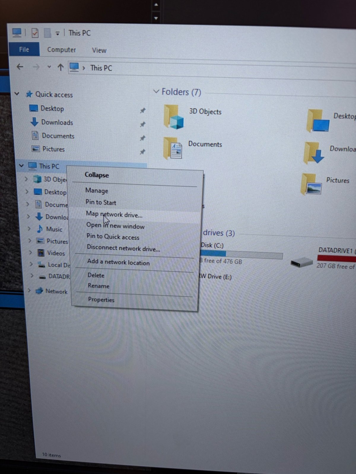
-
-
Enter the share path
-
Set
DrivetoZ:andFolderto\\mallard.stanford.edu\mallard_arina. -
Check
Reconnect at sign-in, then clickFinish. -
Enter the Mallard password when prompted. The password is in the pinned channel of the Colin Ophus group internal Slack.
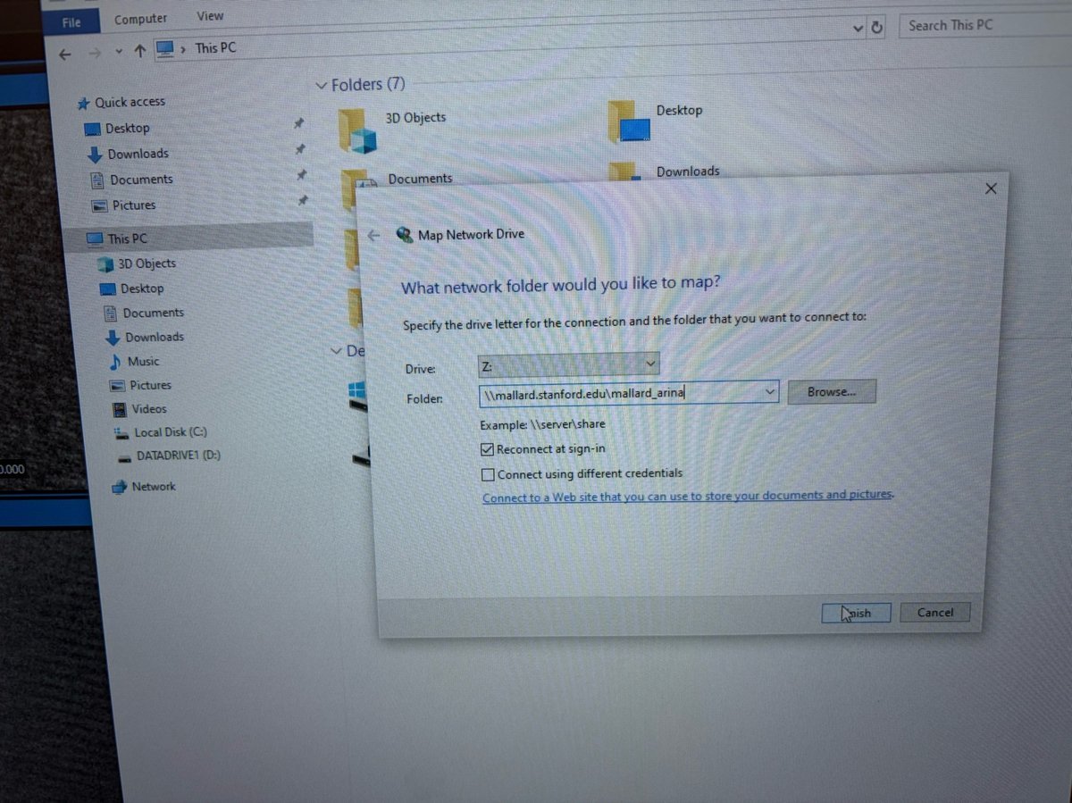
-
Theme 1A & 1B: Spot size and convergence angle (Talos)
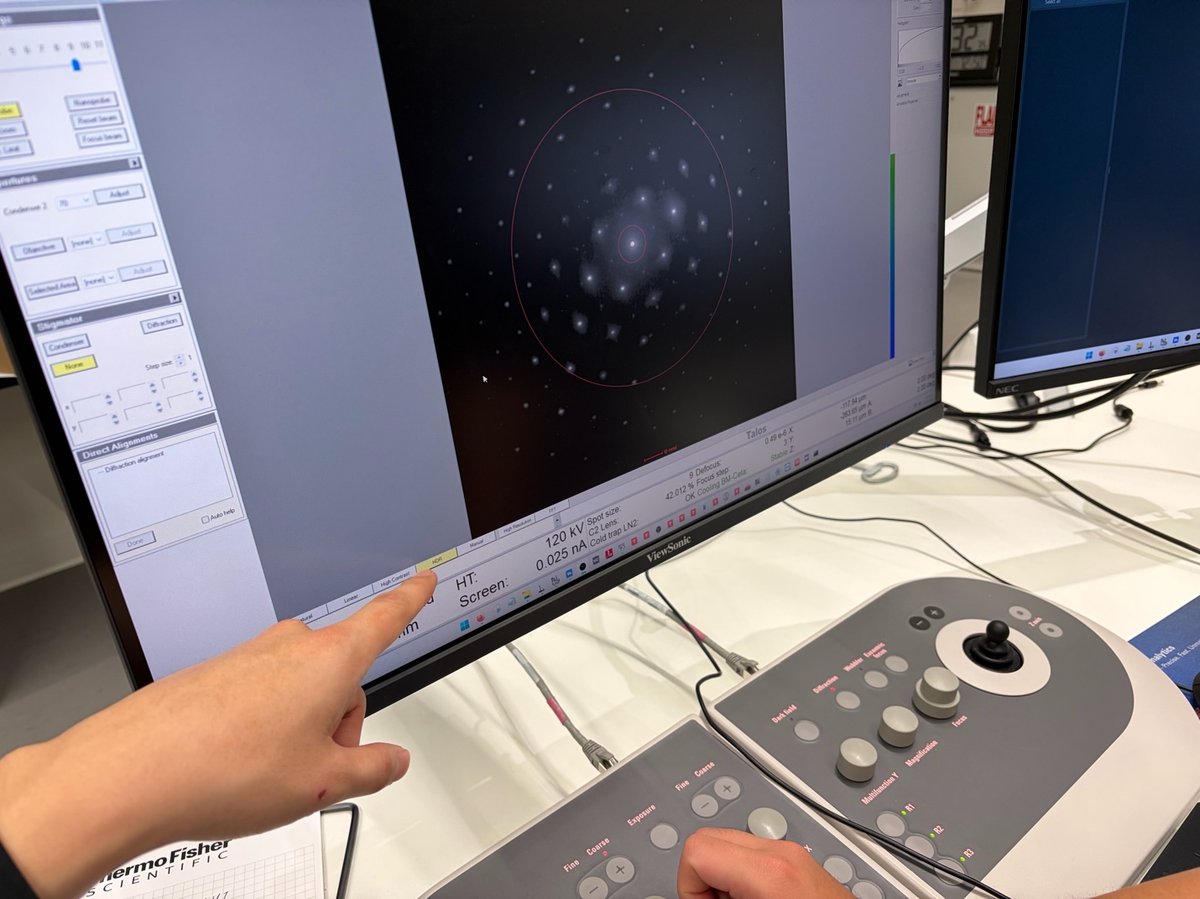
Caution
VERY ROUGH DRAFT, NOT AUTHORITATIVE. Week 3 of the Stanford MATSCI 322 TEM Lab, taught by Andrew Barnum, Pinaki Mukherjee, and Ash. Recorded on 2026-04-21, with an additional underfocus/overfocus session on 2026-04-23. Photos, notes, data, and analysis captured by @bobleesj (Sangjoon Bob Lee) during the sessions as a student. Terminology, step ordering, and values may be wrong or incomplete. Treat this page as a personal study reference, not an SOP. A trained user must verify everything before relying on it.
This lab addresses the following questions:
- How do the spot-size knob and the C2 aperture shape the beam that hits the sample (Theme 1A)?
- How does the C2 lens switch the illumination between parallel, convergent, and defocused, and how does that choice distinguish image mode from diffraction mode (Theme 1B)?
Each section below opens with the specific sub-questions it tackles, then walks through the experiment, the data, and the answer.
Links:
- SNSF Talos reservation / info page: TODO
- Thermo Fisher Talos L120C product page: TODO
System specifications (observed):
| Model | Talos (Thermo Fisher) |
| Accelerating voltage | 120 kV (session value; instrument also supports others) |
| Camera | BM-Ceta |
| C2 apertures tested | 70 µm, 50 µm (handout also lists 150 µm, 100 µm) |
| Probe modes | Microprobe (used in this session), Nanoprobe |
| Magnification range observed | 5,300× (imaging) to 45,000× (for Theme 1B convergent work) |
Acronyms:
C1: first condenser lens (spot-size lens)C2: second condenser lens (intensity / illumination lens)SA: selected areaCL: camera lengthDP: diffraction patternTIA: TEM Imaging and Analysis (Thermo Fisher software)mulXY: multifunction X/Y knobs on the hand panelR1,R3,L3: buttons on the hand control pad (R1 raises/lowers the fluorescent screen; R3 / L3 step spot size up / down)
Overview
| Theme | What you study | Output |
|---|---|---|
| 1A: Beam parameters | Spot size 1–11 × two C2 apertures; record C1, C2, screen current, camera length | Data tables, plots, convergence-angle analysis for lab report |
| 1B: C2 lens & illumination for diffraction | Parallel vs convergent vs defocused beam on oriented gold; lens values in image vs diffraction mode | Lens-value table, C2-condition table, ray diagram sketch |
Theme 1A: How do spot size and C2 aperture shape the beam?
What this section addresses
The beam that reaches the sample is the product of two things: the condenser lens system (C1 sets the spot size, C2 sets the illumination) and the condenser aperture selection. Three sub-questions to answer:
- When the spot-size knob is stepped, what actually moves? Only C1? Or C2 as well?
- The intensity knob clearly moves C2. Does it move C1 too?
- How much does the aperture change matter? Is a 70 µm aperture really that different from 50 µm at the same spot size?
Diffraction camera length for a 5 mm beam
| Spot size | CL at 70 µm C2 | CL at 50 µm C2 |
|---|---|---|
| 3 | 1.75 m | 2.2 m |
| 9 | 1.75 m | 2.21 m (recovered from Ceta .emd metadata; not measured directly with the 5 mm marking) |
Plots

What did the data tell us?
- Spot size drives C1, not C2. C1 swings from ~17% at spot 1 to ~93% at spot 11, a factor of 5. C2 drifts from ~44.5% to ~39%, only about 5 percentage points.
- The aperture barely moves the lenses. The 70 µm and 50 µm curves sit on top of each other in both C1 and C2 plots. The aperture clips the beam; it doesn’t reshape the lens system.
- The intensity knob moves C2 but not C1 (confirmed by watching the System Status panel while turning intensity).
- Screen current drops by ~200× from spot 1 to spot 9 at fixed aperture (5.80 nA → 0.030 nA on the 70 µm curve), approximately exponential on the log-y plot (about a factor of two per step).
- 70 µm delivers ~2× the screen current of 50 µm at every spot above the detection limit. The area ratio is (70/50)² ≈ 2, which matches: the aperture really is just clipping.
- A 5 mm beam needs longer camera length at 50 µm C2. At spot 3: 1.75 m (70 µm) vs 2.2 m (50 µm). Less beam, so more camera length is needed to magnify it to the same ring.
How big is the convergence angle, and what sets it?
In diffraction mode the focused-probe central disk has angular radius equal to α. With the disk set to fill the inner 5 mm screen marking (small-angle limit, α = 2.5 mm / L):
| C2 aperture | Spot | Camera length L | α = 2.5 mm / L |
|---|---|---|---|
| 70 µm | 3 | 1.75 m | 1.43 mrad |
| 70 µm | 9 | 1.75 m | 1.43 mrad |
| 50 µm | 3 | 2.20 m | 1.14 mrad |
| 50 µm | 9 | 2.21 m | 1.13 mrad |
The result. α is set by the C2 aperture, not by spot size. At a given aperture, α is the same at spot 3 and spot 9. Going from 70 µm to 50 µm at spot 3 reduces α from 1.43 to 1.14 mrad. The 50 µm aperture clips the convergent cone to a smaller half-angle.
Why doesn’t spot size affect α? (ray diagram)
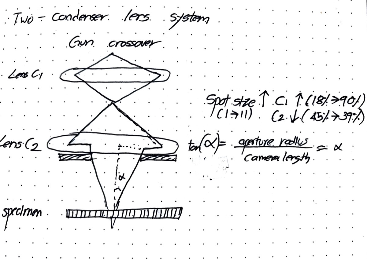
The electron beam travels down the column in this order: it starts at the gun crossover, passes through the C1 lens, forms an intermediate crossover, gets clipped by the C2 aperture, passes through the C2 lens, and lands on the specimen.
The spot-size knob only changes how strongly C1 is excited. Turning C1 up shortens its focal length, which shrinks the image of the gun crossover that arrives at the C2 aperture. A more shrunken crossover means a smaller, dimmer probe on the specimen.
What the spot size cannot change is the C2 aperture radius (r_ap). The aperture is a physical disk with a fixed hole, so it always clips the converging cone to the same radius. C2 then projects that cone onto the specimen at a fixed distance away. Putting these two together: the convergence half-angle α at the specimen is set by the aperture radius and that fixed C2-to-specimen distance, and is independent of the spot size. In the small-angle limit, tan(α) ≈ α = r_ap / L.
Why is C1 so low at spot 1?
Spot 1 wants the largest probe and the highest current, which means the least demagnification of the gun crossover. C1 at minimum strength does the least demagnification, hence the very low percentage at spot 1. As the spot number increases, more demagnification is requested, so C1 % climbs.
Why does one camera length cover both spot 3 and spot 9?
The 5 mm-beam method sets the focused-probe central disk equal to the 5 mm screen ring. Disk radius = α × L. Because α is fixed by the C2 aperture (independent of spot size), a single L gives the 5 mm condition for every spot at that aperture. The 50 µm aperture has a smaller α, so a larger L (2.2 m vs 1.75 m) is needed to inflate its disk back to 5 mm.
Theme 1B: How does the C2 lens switch between parallel and convergent illumination?
What this section addresses
Theme 1A focused on the beam at crossover. But the beam has more states than that: it can be parallel, convergent to a point, or defocused on either side of crossover. Each state changes what the sample sees, and the switch between image mode and diffraction mode on a TEM is really just a choice of which lenses are doing what.
Two sub-questions to answer:
- When the instrument switches between imaging and diffraction modes, which lenses actually change values? Is it really a C2 thing, or do the post-sample lenses do the heavy lifting?
- What does the beam at the sample look like when defocused clockwise vs counter-clockwise through crossover? Are the two sides symmetric, or does something meaningful change?
The sample is a commercially-available oriented gold standard: evaporated to ~11 nm, (100) orientation, loaded in a double-tilt holder and aligned to its zone axis before the session started.
Experimental setup
Two sub-experiments.
Experiment 1: lens values in image vs diffraction mode. At 5,300× magnification with C2 = 70 µm and spot size 9, the beam is expanded clockwise through crossover until the diffraction pattern becomes sharp (parallel illumination). The four post-sample lens values (Diffraction, Intermediate, Projector 1, Projector 2) are recorded from the System Status panel in image mode, then again after switching to diffraction mode with CL = 420 mm.
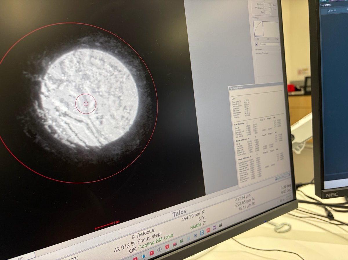
Experiment 2: sweeping through crossover. Camera length is increased to 2.2 m and magnification to 45,000×. The beam is focused to a point on the phosphor, and the central disk is centered with mulXY. The intensity knob is then turned clockwise from the focused point until features reappear inside the central disk; next, counter-clockwise through crossover and past it until features reappear on the other side. An image is acquired at each stopping point, along with the C2 value.
Note: if the phosphor screen “flaps” when
R1is pressed, press again until it settles in the desired position. This is normal instrument behavior.
Which lenses change between image mode and diffraction mode?
| Lens | Image mode (%) | Diffraction mode (%) |
|---|---|---|
| Diffraction | 44.65 | 28.42 |
| Intermediate | -14.81 | -0.281 |
| Projector 1 | 41.81 | 52.84 |
| Projector 2 | 97.09 | 98.07 |
How does the beam change as C2 is swept through crossover?
The successive states the beam passes through during Experiment 2, read top to bottom along the C2 knob:
- Parallel (start): beam expanded post-crossover, diffraction pattern sharp, C2 = 42.01%.
- Convergent (at crossover): C2 turned clockwise into crossover so the beam focuses to a point on the phosphor. Central disk is featureless with only a few scattered spots. This is the reference point for the defocus sweep.
- Defocused clockwise from focus: from crossover, C2 is nudged further clockwise (slightly stronger) until features reappear inside the central disk. C2 = 40.06%, beam diameter ≈ 1.28 µm.
- Back through focus, then defocused counter-clockwise: C2 is rotated counter-clockwise past crossover until features appear again. C2 = 38.663%, beam diameter ≈ 1.39 µm. Features look the same as in step 3, but the real-space orientation is flipped.
The full table with FluCam image-mode and diffraction-mode captures for each of these conditions is in the FluCam screenshots section below.
The C2 values for steps 3 and 4 straddle the crossover value (39.396%) by roughly ±0.7 percentage points in either direction. The ~0.7% offset is how far the intensity knob had to travel past crossover before the central disk showed features again.
What did the data tell us?
- Switching image to diffraction mode moves every post-sample lens, with the Intermediate lens doing the actual mode switch. Diffraction lens 44.65 → 28.42%, Intermediate −14.81 → −0.281%, Projector 1 41.81 → 52.84%, Projector 2 essentially unchanged. The full mechanism is in the Ray diagrams section below.
- C2 values for each beam condition are close but not identical. Parallel at 5,300× is C2 = 42.01%. Convergent (beam focused to a point) at 45,000× is C2 = 39.396%. Defocused on either side of crossover is ±1% around the crossover value.
- Defocus clockwise and counter-clockwise through crossover produce images that look the same, but are flipped in real space. Past crossover, the beam inverts: features you saw on the left end up on the right.
- Short camera length = wider diffraction view; long camera length = tighter central disk. At 350 mm CL many Bragg peaks fit on screen; at 2.2 m CL only the central disk and nearest reflections fit.
- Thermo Fisher’s mental model: the beam is the reference point. Start from parallel illumination in image mode; watching how the beam converges or diverges as you adjust C2 is how you reason about every other mode.
How do the same lenses produce both an image and a diffraction pattern?
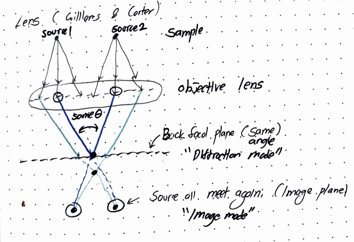
Two sample sources emit fans of parallel-illumination rays. The objective lens has two natural conjugate planes downstream:
- At the back focal plane, rays of the same exit angle (regardless of which source they came from) focus to one point. That is the diffraction pattern.
- At the image plane (further down), rays from the same source (regardless of exit angle) focus to one point. That is the real-space image.
The objective is unchanged between the two modes; what switches is the intermediate lens, which re-focuses the camera onto either the back focal plane (diffraction mode) or the image plane (image mode). The lens-excitation table above shows this directly: the intermediate lens swings from −14.81% to −0.281% while the objective stays put.
The “Diffraction lens” name is misleading. It is the first projection lens after the objective, not a lens that is only on in diffraction mode. It actually gets weaker in diffraction mode (44.65% → 28.42%) because once the intermediate lens drops out, Projector 1 takes over and gets stronger; the chain has one fewer stage to do work, so the Diffraction lens slackens.
Does Bragg’s law agree with the displayed camera length?
The Ceta .emd files carry the full FEI metadata (acceleration voltage, camera length, lens excitations, pixel scale). For the Ceta diffraction acquisitions taken in this session: HT = 120 kV, spot index = 9, C1 = 51.85% (matching the 50 µm aperture spot 9 row of the data table), camera lengths = 2.209 m (#0015–17) and 1.065 m (#0018–21). The 70 µm aperture was not used during the Ceta diffraction acquisitions.
Relativistic wavelength (λ = h·c / √(eV·(eV + 2 m_e c²))):
| HT | λ (pm) |
|---|---|
| 120 kV (this session) | 3.35 |
| 200 kV | 2.51 |
| 300 kV | 1.97 |
Bragg angle for gold {200} (d_200 = a/2 = 0.2035 nm; small-angle: 2θ_B ≈ λ/d):
| HT | 2θ_B for {200} (mrad) |
|---|---|
| 120 kV | 16.5 |
| 200 kV | 12.3 |
| 300 kV | 9.7 |
True camera length from the {200} reflection. Using the Velox pixel scale (0.01628 1/nm/pixel for L = 1.065 m), the {200} spot lies at q = 1/d_200 = 4.91 1/nm, which is 4.91 / 0.01628 = 302 pixels from the central beam. With effective pixel size 56 µm, this is 302 × 56 µm = 16.9 mm. Then L_true = 16.9 mm / 16.5 mrad = 1.024 m. For #0015–17 the same calibration gives L_true ≈ 2.221 m.
Comparison of displayed vs metadata vs Bragg-back-calculated camera length:
| Capture | L displayed (m) | L from .emd metadata (m) | L calculated from {200} Bragg (m) | Agreement |
|---|---|---|---|---|
| #0015–17 | 2.20 | 2.209 | 2.221 | within 1% |
| #0018–21 | 1.05 | 1.065 | 1.024 | within 4% |
All three agree within ~4%, which is the expected calibration accuracy for the Talos camera-length setting.
True convergence angle. The 5 mm-marking measurement on the 50 µm aperture was made at L = 2.20 m, so the matching Bragg-calibrated camera length is L_true = 2.221 m (from #0015–17). Then α_true = 2.5 mm / 2221 mm ≈ 1.13 mrad, in agreement with the screen-marking value of 1.14 mrad to within 1%.
What is the effective Ceta pixel size at 120 kV vs 300 kV?
The Ceta has 14 µm physical pixels. With binning 4 the output frame is 1024 × 1024 with effective pixel = 56 µm. The real-space pixel size at the specimen depends on imaging mode (microprobe vs nanoprobe) and magnification, not on HT directly: HT only changes the wavelength (and therefore the reciprocal-space pixel scale in diffraction mode). For the Ceta in diffraction mode at L = 1.065 m:
- At 120 kV (λ = 3.35 pm), reciprocal pixel = 56 µm / (1065 mm × 0.00335 nm) = 0.0157 1/nm/px. Velox-reported pixel scale: 0.01628 1/nm/px (3.7% disagreement, consistent with the camera-length calibration above).
- At 300 kV (λ = 1.97 pm), reciprocal pixel = 56 µm / (1065 mm × 0.00197 nm) = 0.0267 1/nm/px (predicted; not measured this session).
Higher kV covers more reciprocal space per pixel at the same camera length (each pixel spans more 1/nm), so more Bragg orders fit in the camera FOV, at the cost of coarser q resolution per pixel.
Why does longer camera length show fewer Bragg spots?
Camera length in a TEM behaves like the throw distance of a movie projector:
- Move the projector close to the wall (short L): the image on the wall is small, but the whole picture fits.
- Move the projector far from the wall (long L): the image on the wall is huge, but only the center fits in view.
Diffraction mode works the same way. Every Bragg spot sits at a fixed angle 2θ from the center; on the camera it lands at r_on_camera = 2θ × L.
- Long L (2.20 m): each Bragg spot is far from center, the pattern is spread out, and the fixed-size camera only catches the central disk plus maybe one reflection (Ceta capture below at 1 nm⁻¹ scale).
- Short L (1.05 m): spots land closer to center, more spots squeeze inside the camera, and the gold (100) zone-axis spots start to appear (Ceta capture below at 5 nm⁻¹ scale).
- Very short L (350 mm, observed in 1B but not recorded with the Ceta): many Bragg orders fit at once, ideal for whole-pattern overviews.
So long L means “magnify reciprocal space” (good for measuring α from the central disk against a screen marking); short L means “wide-angle reciprocal view” (good for seeing the whole pattern at once).
| L = 2.20 m (focused central disk) | L = 1.05 m (focused central disk with gold {200} spots in view) |
|---|---|
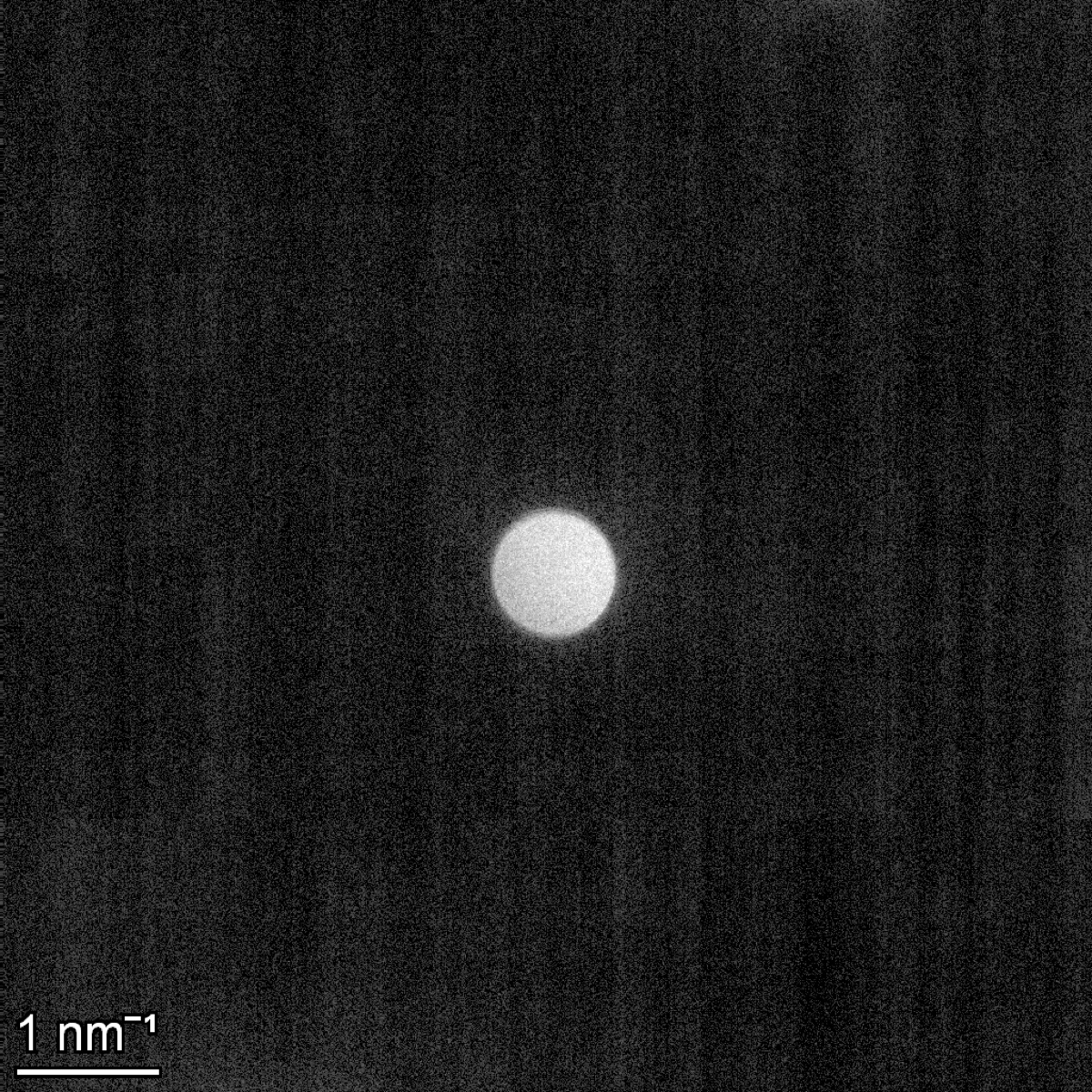 |
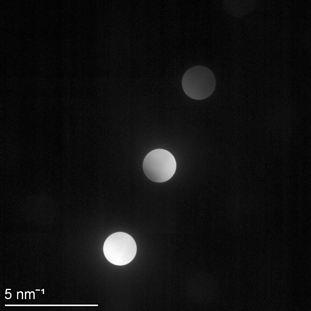 |
Can the over- vs under-focus flip be seen directly on the Ceta?
The two Ceta captures below were taken at L = 2.20 m on opposite sides of the focused crossover. The diagonal dark band inside the disk shifts/inverts between the two, while the outer disk geometry (set by the C2 aperture) is unchanged. This is the over/under-focus contrast inversion (sign change in the contrast transfer function), shown here in the central disk itself rather than in the real-space image.
| L = 2.20 m, defocused side A (#0016) | L = 2.20 m, defocused side B (#0017) |
|---|---|
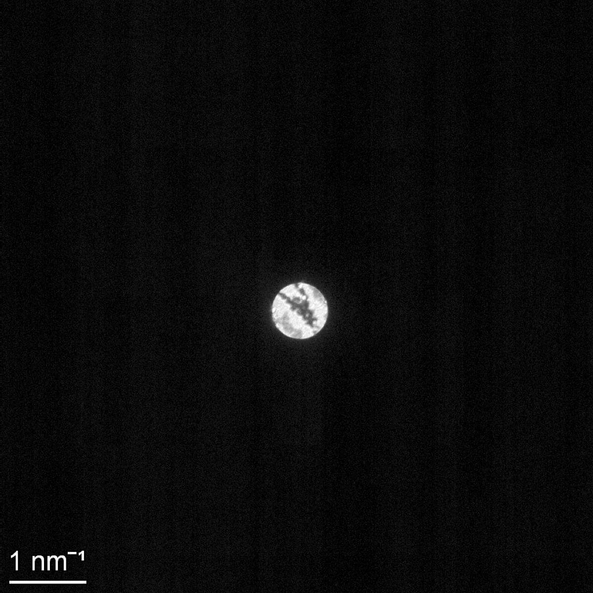 |
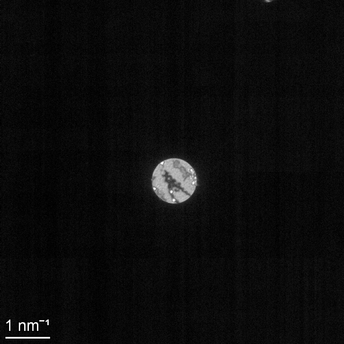 |
What does each C2 condition look like on the FluCam?
The four C2 conditions from the lab table mapped to the FluCam captures (image mode and diffraction mode for each). Image/diffraction mode classification comes from the .emi ObjectInfo (Real Space vs Reciprocal Space); the four conditions were mapped to the eight tifs by combining the timestamp order of the .emi files (procedure flow: Parallel → Convergent → Defocused #1 → Defocused #2) with the visible scale bar and probe geometry in each tif. The Parallel and Convergent assignments are unambiguous from the beam diameter; the Defocused #1 vs #2 pairing is inferred from chronological order (the per-tif .ser metadata was not in the folder).
| C2 condition | Mag | C2 (%) | Beam diameter | Camera length | Image mode (FluCam) | Diffraction mode (FluCam) |
|---|---|---|---|---|---|---|
| Parallel | 5,300× | 42.01 | 5.25 µm | 420 mm | 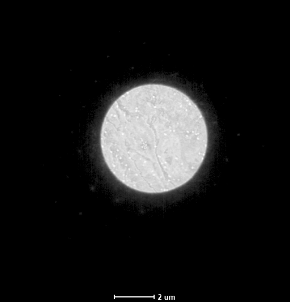 tif 3 · 2 µm scale |
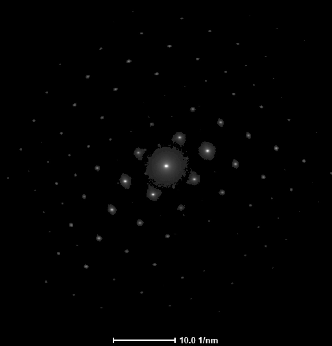 tif 2 · 10.0 1/nm |
| Convergent (focused crossover) | 45,000× | 39.396 | 73 nm | 2.2 m | 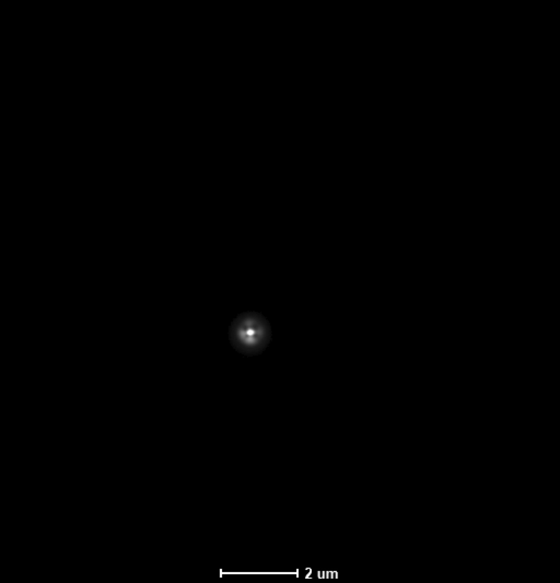 tif 8 · 2 µm scale |
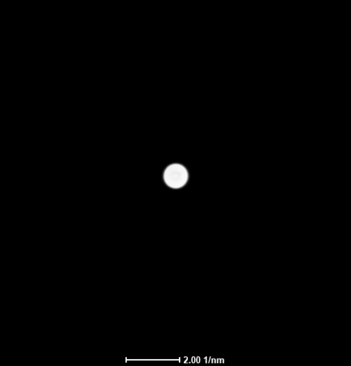 tif 1 · 2.00 1/nm |
| Defocused #1 (intensity knob clockwise from convergent, C2 up) | 45,000× | 40.06 | 1.28 µm | 2.2 m | 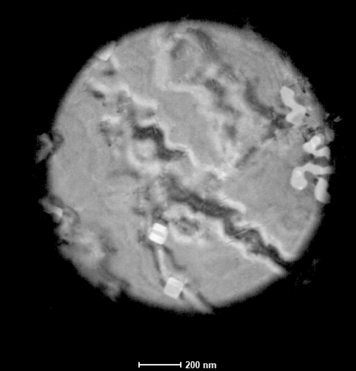 tif 6 · 200 nm scale |
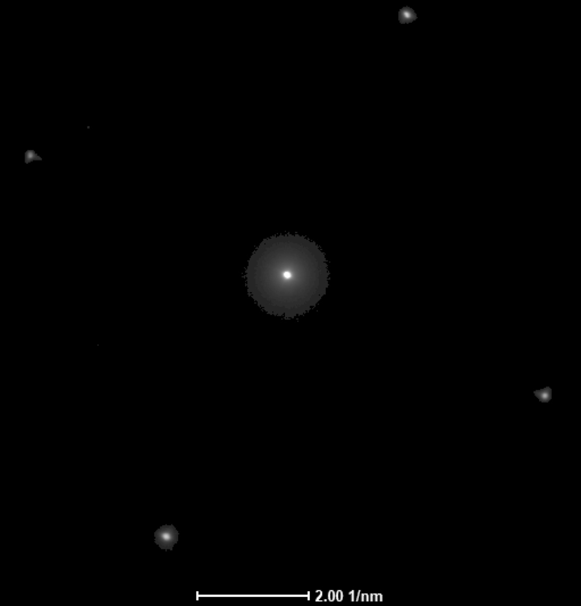 tif 4 · 2.00 1/nm |
| Defocused #2 (intensity knob counter-clockwise from convergent, C2 down) | 45,000× | 38.663 | 1.39 µm | 2.2 m | 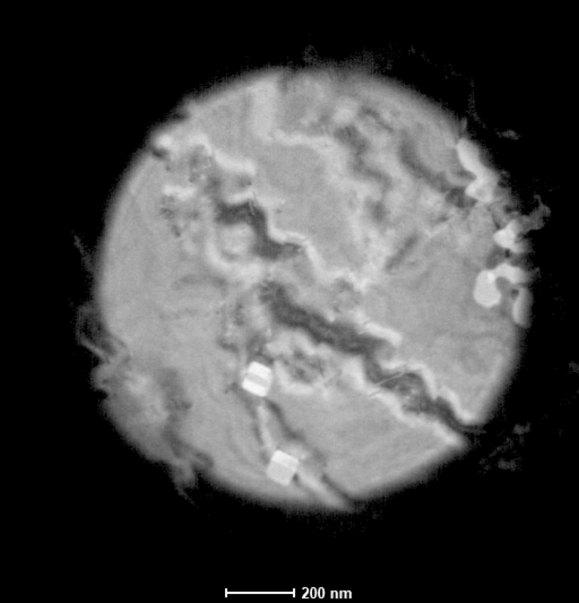 tif 7 · 200 nm scale |
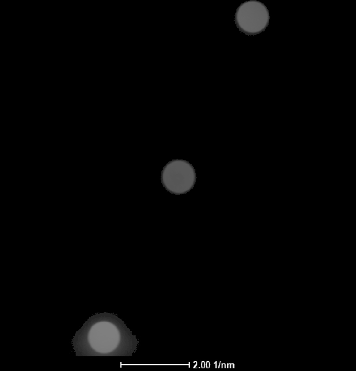 tif 5 · 2.00 1/nm |
Stepping through Defocused #1 → Convergent → Defocused #2 sweeps the intensity knob through the focused crossover. The two defocused image-mode probes (tif 6 vs tif 7) cover the same sample area but show inverted internal contrast; the two defocused diffraction-mode disks (tif 4 vs tif 5) similarly flip their internal fringes. Whether the “C2 up” side corresponds to true overfocus or underfocus depends on whether the C2-lens perspective or the beam perspective is being used (these conventions are opposite).
Why does the image flip when defocus crosses zero?
When the beam crossover sits above the sample plane (over-focus), the rays have already crossed by the time they reach the sample, so left/right is inverted on the specimen. When the crossover sits below the sample plane (under-focus), the rays have not crossed yet, so the orientation is preserved. Stepping the intensity knob through crossover swaps over- and under-focus, hence the real-space flip.
Changelog
- May 11, 2026 : Filled in the Theme 1A and Theme 1B analysis (convergence angle, two-condenser ray diagram, Williams and Carter ray diagram, Bragg’s law verification of camera length, comparison to displayed and
.emdmetadata values, effective real-space pixel calculation). Recovered the spot 9 / 50 µm camera length from the Ceta.emdmetadata. Added a brief reference to the over/under-focus session of 2026-04-23. - Apr 22, 2026 : Initial draft from the 2026-04-21 Week 3 TEM class lab taught by Andrew B. Photos, notes, and measurements by @bobleesj. Plots generated from the xlsx data sheet. Analysis prompts and ray diagrams left as TODO for the lab report.
Theme 1C: SEM and STEM imaging (Phenom Pharos)
****# Phenom Pharos G2 SEM/STEM (Deep Lab)
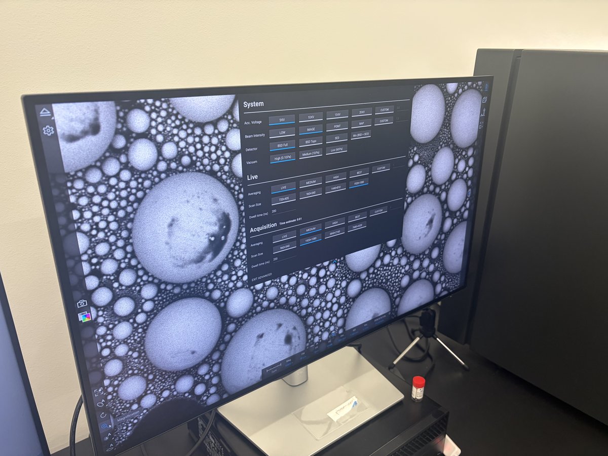
Caution
VERY ROUGH DRAFT - Notes and photos recorded by @bobleesj during TA session with Ash on Apr 16, 2026. Based on the Theme 1C “Imaging Basics on the Phenom” lab walkthrough. The goal of this guide is to help you operate the Phenom Pharos in the future, not to reproduce the lab exercise. Steps and screenshots still need verification.
TODO: Further verify every step against the actual instrument. Add screenshots for tuning buttons (autofocus, autoCB, autostigmate) and the accelerating voltage / detector / vacuum selectors.
This guide covers operating the Phenom Pharos G2 desktop SEM/STEM in the Deep Lab at Stanford. The Phenom Pharos is a desktop-sized field-emission SEM that also supports STEM imaging through a swappable holder. It is fast to start up (no pump-down wait like the Spectra), and the UI is simple enough that a new user can be imaging within a few minutes.
Links:
System specifications:
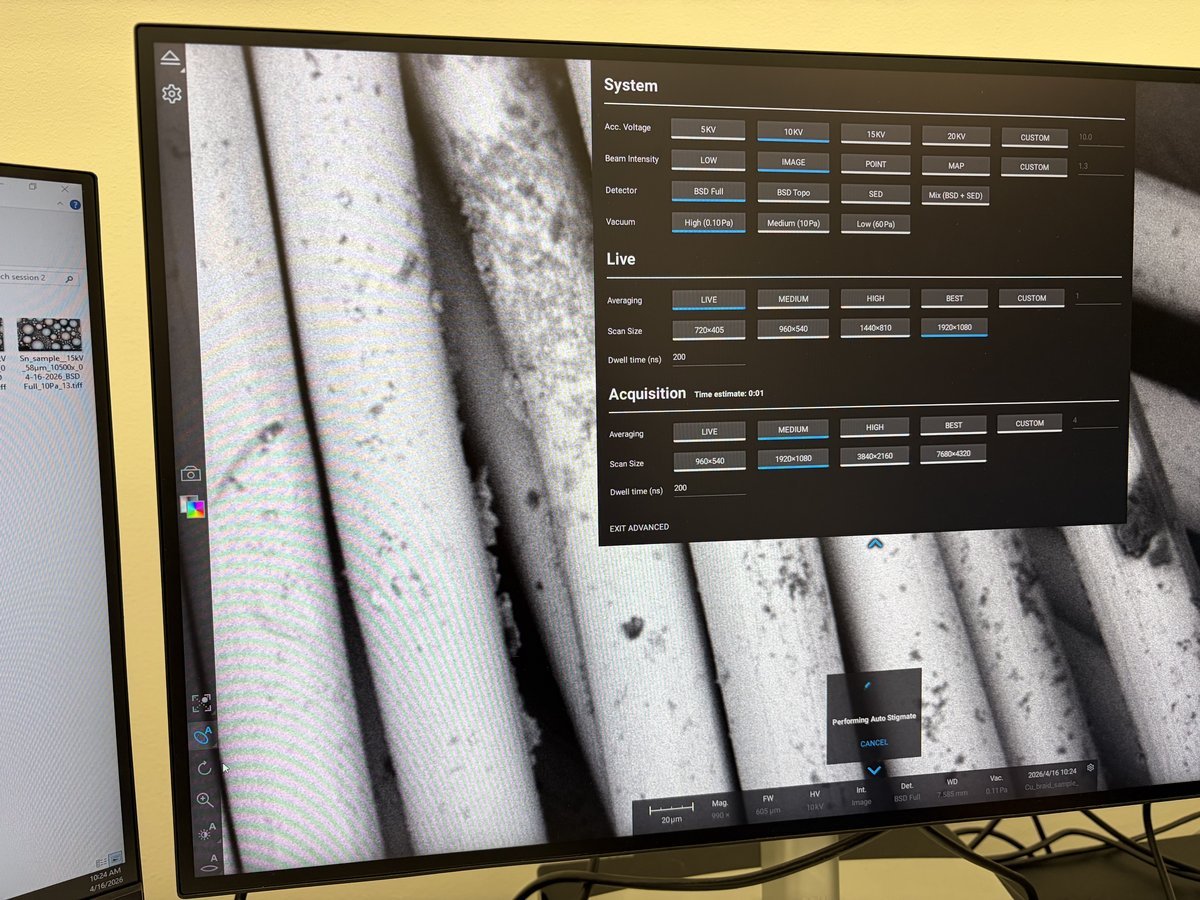
The acquisition settings panel shows what is available: accelerating voltage (5/10/15/20 kV or custom), beam intensity (Low/Image/Point/Map/Custom), detector (BSD Full, BSD Top, SED, or 4A+BSD+SED), and vacuum (High 0.1 Pa, Medium 10 Pa, Low 60 Pa).
| Model | Phenom Pharos G2 Desktop FEG-SEM |
| Source | Schottky field emission |
| Sample size | 25 mm max diameter |
| Resolution | SED: 2 nm, STEM: <1 nm |
| Detectors | SED, BSD (BSE), BSD-TOPO, EDS, STEM (BF, DF, HAADF) |
| Acceleration voltage | 1 to 20 kV |
| Vacuum | 0.1 Pa, 1 Pa, 60 Pa (low/medium/high) |
| Footprint | 925 × 305.6 × 343.5 mm, 83.8 kg |
Acronyms:
SEM- Scanning Electron Microscopy (surface imaging)STEM- Scanning Transmission Electron Microscopy (thin-sample imaging)SED- Secondary Electron Detector (surface topography)BSD/BSE- Backscattered Electron Detector (atomic number contrast)BF/DF/HAADF- Bright Field / Dark Field / High-Angle Annular Dark Field (STEM modes)autoCB- Auto Contrast-BrightnessWD- Working DistanceFW- Field Width
Example images produced by the Phenom Pharos:
- Secondary electron image of tin on carbon standard (SED mode)
- STEM bright field image of rubber sample (BF STEM mode)
Overview
| Phase | What it covers | Time |
|---|---|---|
| Part 1: Loading a sample | Prepare sample on stub puck, insert into drawer | 5 min |
| Part 2: Transfer to SEM | Optical overview, set accelerating voltage, move to SEM | 2-3 min |
| Part 3: Imaging and tuning | Pick magnification, autofocus/autoCB/autostigmate, acquire images | varies |
| Part 4: Maps software for large-area tiles | Switch to Maps software, set up a tile series | 5-15 min |
| Part 5: STEM mode | Swap to STEM holder, load a TEM grid, image in BF/DF/HAADF | 15-30 min |
| Part 6: End session | Save images, unload sample, hand off | 5 min |
Part 1: Loading sample
1.1 Unload sample
-
Eject and open the drawer
-
Put on nitrile gloves before handling any sample or holder.
-
In the software, click the eject icon (triangle in the left sidebar) to vent the chamber. Wait for the vent cycle to finish.
-
Pull the bottom drawer on the front of the Phenom Pharos G2 open.
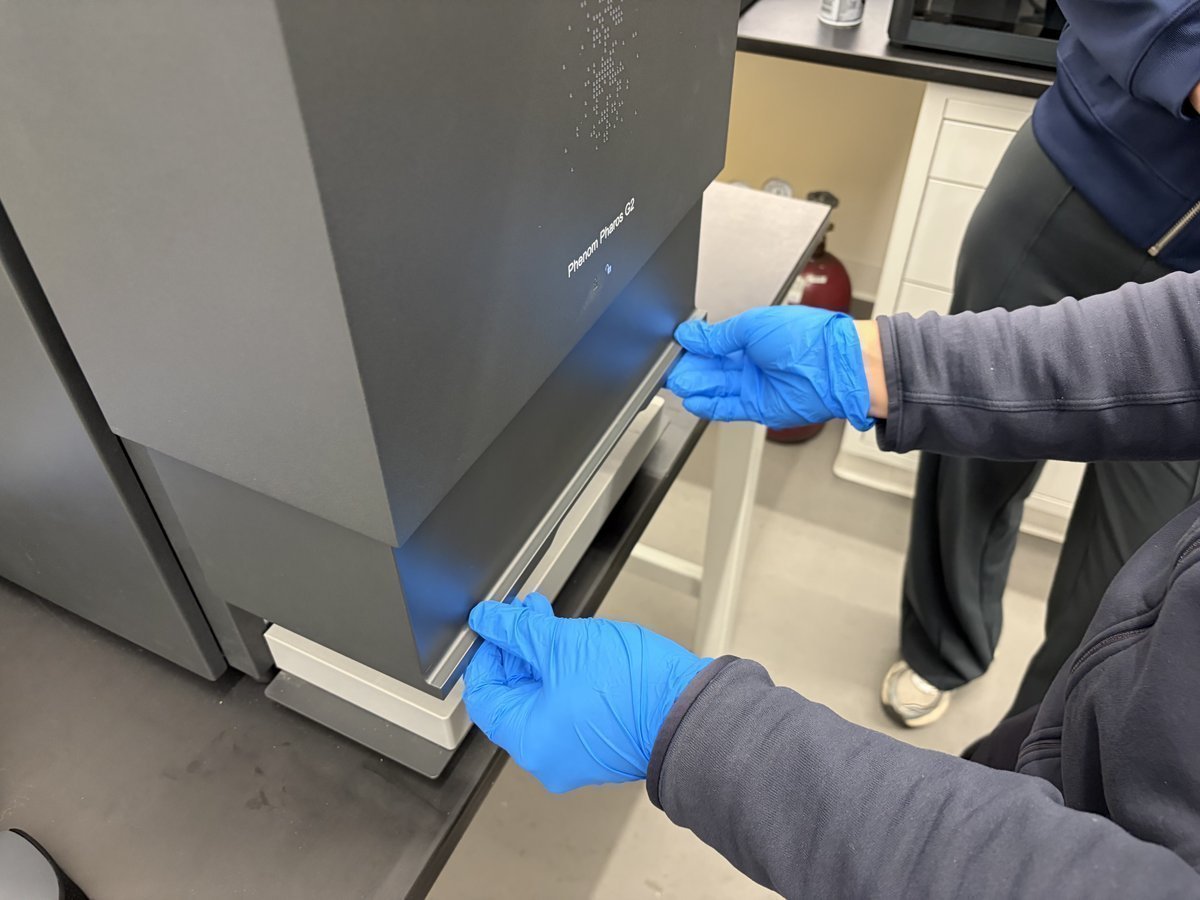
-
-
Remove the existing stub
-
The previous user’s stub puck is seated in the drawer. Lift it out by the black handle.
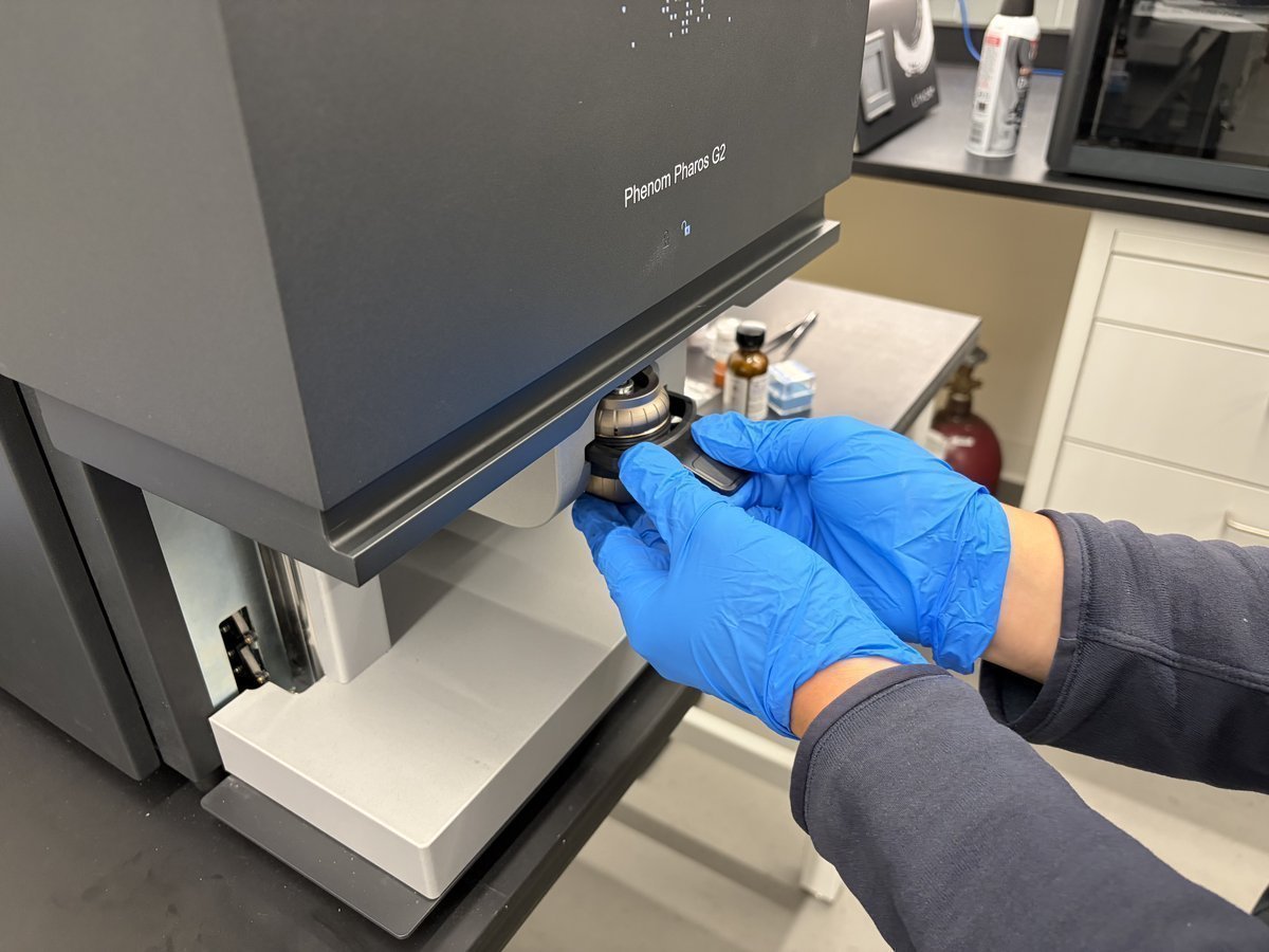
-
Gently pull it out
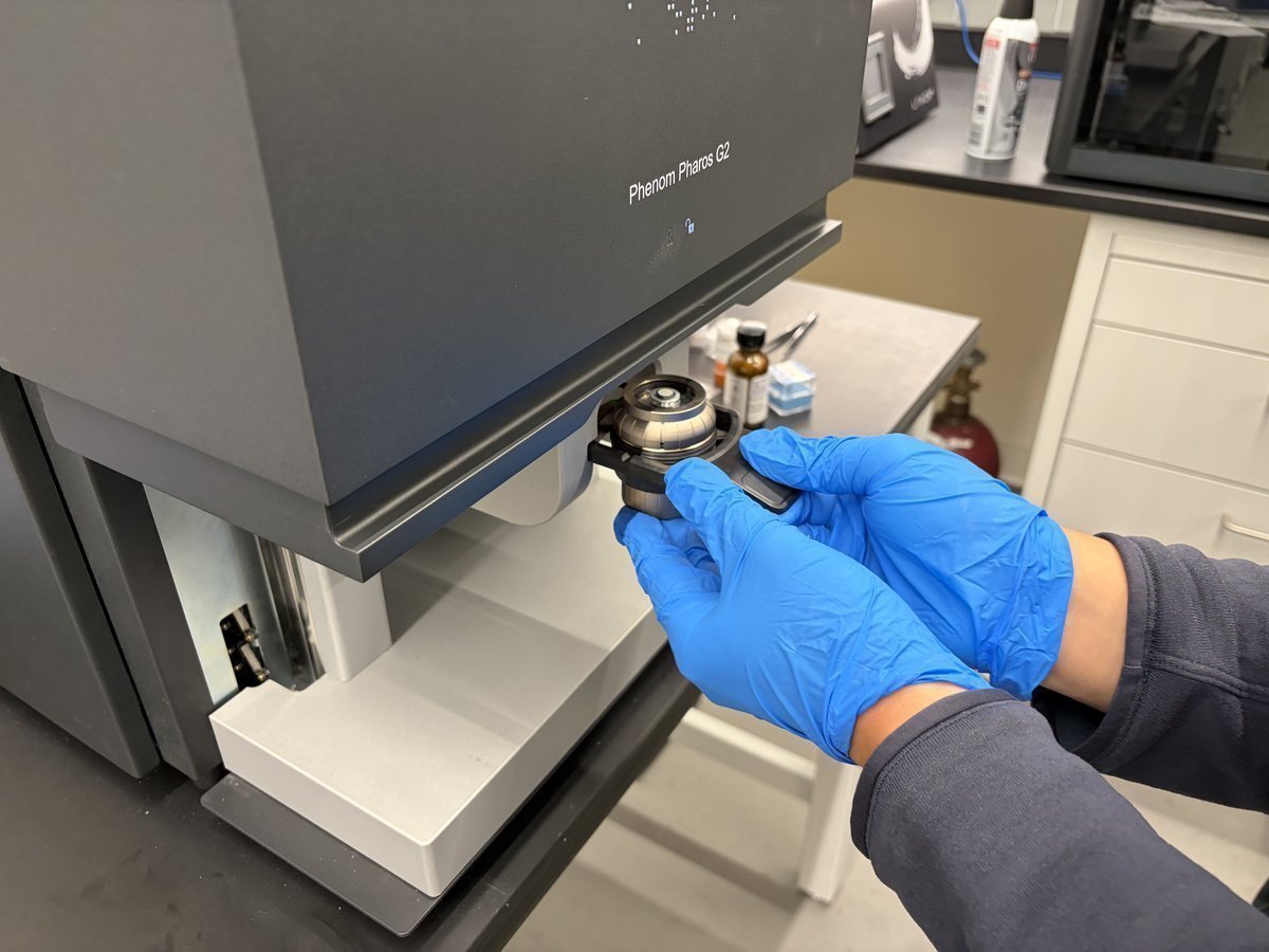
-
-
Remove the old sample
-
Use a tweezer to pick the previous sample off the stub.
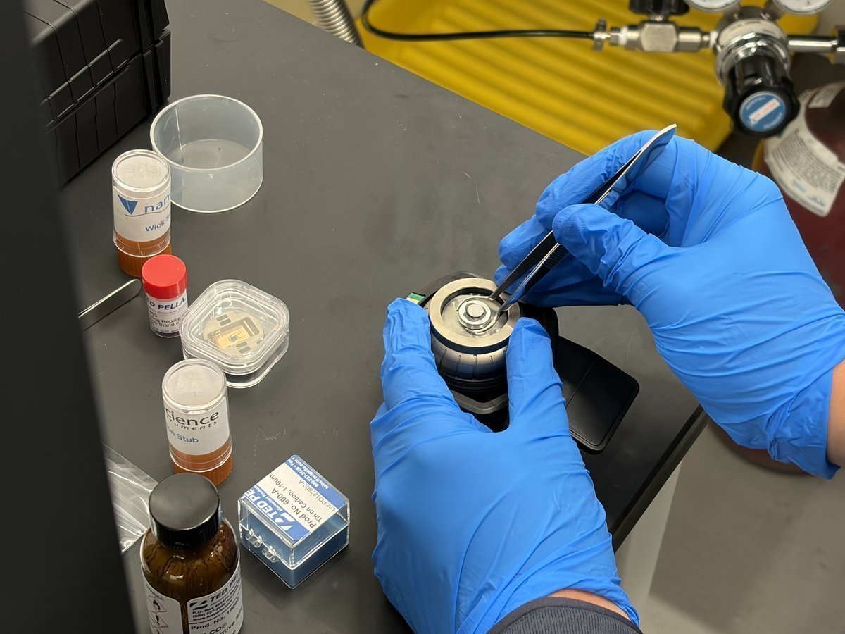
-
Lift the sample clear of the stub. The stub center is now empty.
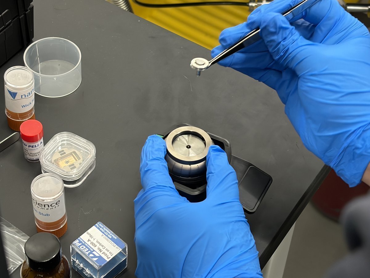
-
Place the old sample aside on the bench. You can return it to its storage tube at the end of the session.
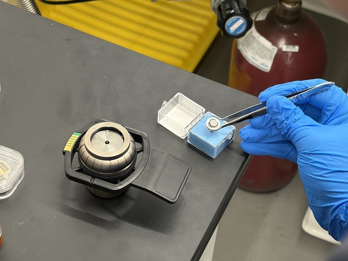
-
1.2 Load your sample
-
Get your new sample from its orange tube
-
Locate the orange-capped storage tube labeled with your sample name (for example,
Cu braid). -
Uncap the tube and use the tweezer to reach for your new sample inside.
-
Lift the new sample out of the tube by its edge.
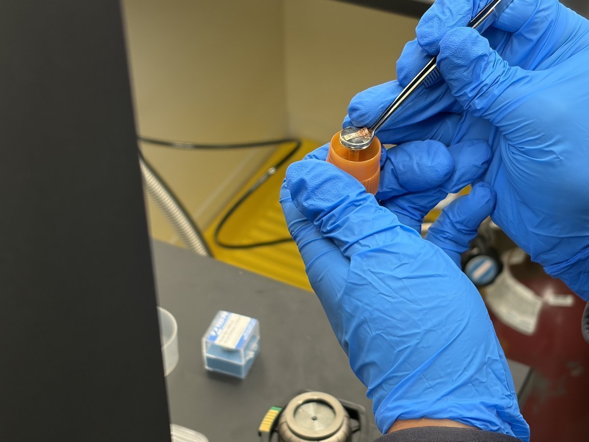
-
-
Bring the sample to the stub
-
With the stub empty in hand, position the new sample above the stub center.
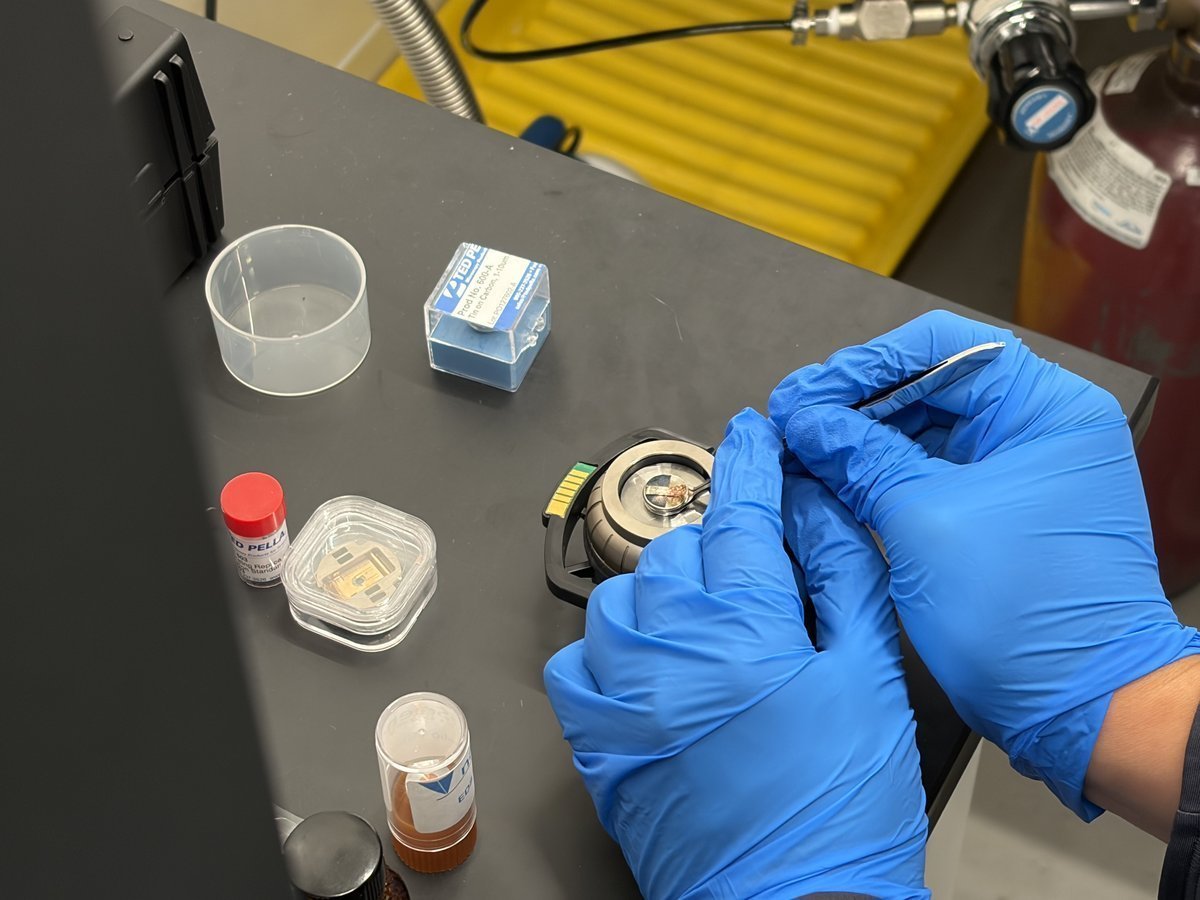
-
-
Place and secure the sample
-
Lower the sample onto the center of the stub.
-
If needed, press down firmly with your thumb to secure the sample against the stub.
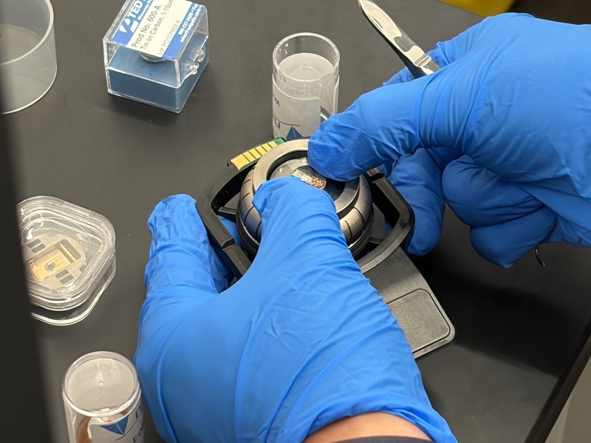
-
-
Verify the mounted sample
-
Hold the stub up and inspect from the side. The sample must sit below the metal rim and be centered.
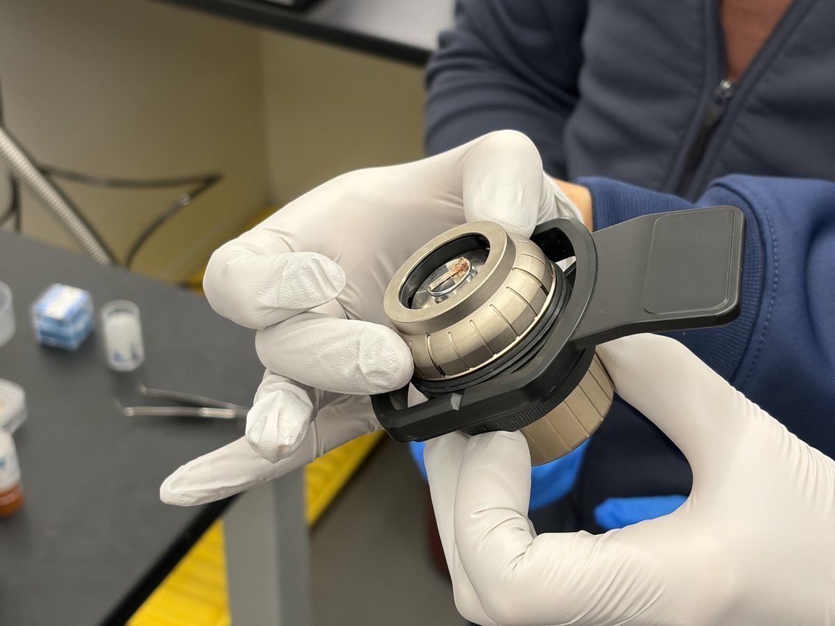
CRITICAL: If the sample sticks above the rim, it will hit the pole piece when the stage raises. Flatten or reseat before inserting.
-
1.3 Insert and close the drawer
-
Lift up the drawer and insert the stub. The Phenom begins pumping down automatically. The front display shows a loading animation while pumping. Wait for pumping to complete before proceeding.
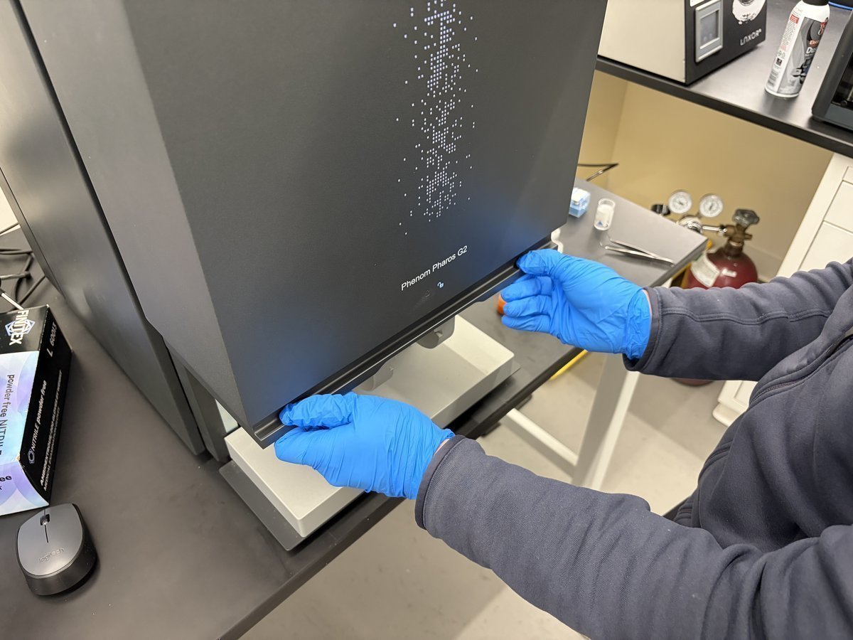
Part 2: Transfer to SEM
2.1 View the optical overview
When the drawer closes and pumping completes, the Phenom starts in optical mode. You see the sample through the loading camera, not the electron beam yet.
NOTE: The mouse scroll wheel behaves differently in each mode:
- Optical mode (first load): scroll adjusts optical focus.
- SEM mode (after “Move to SEM”): scroll adjusts magnification.
Don’t expect to zoom with the wheel until you move to SEM.
-
See the optical camera view
-
The software shows the optical view of your sample from the loading camera. Use this to get a rough idea of where your features are on the stub.
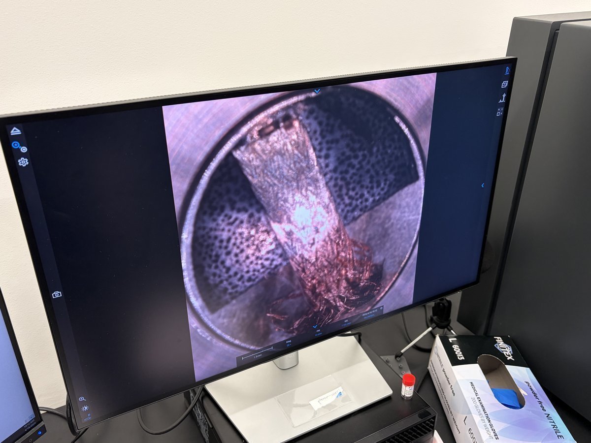
-
Scroll the mouse wheel to focus the optical camera. The optical view is useful for orientation but cannot resolve fine features.
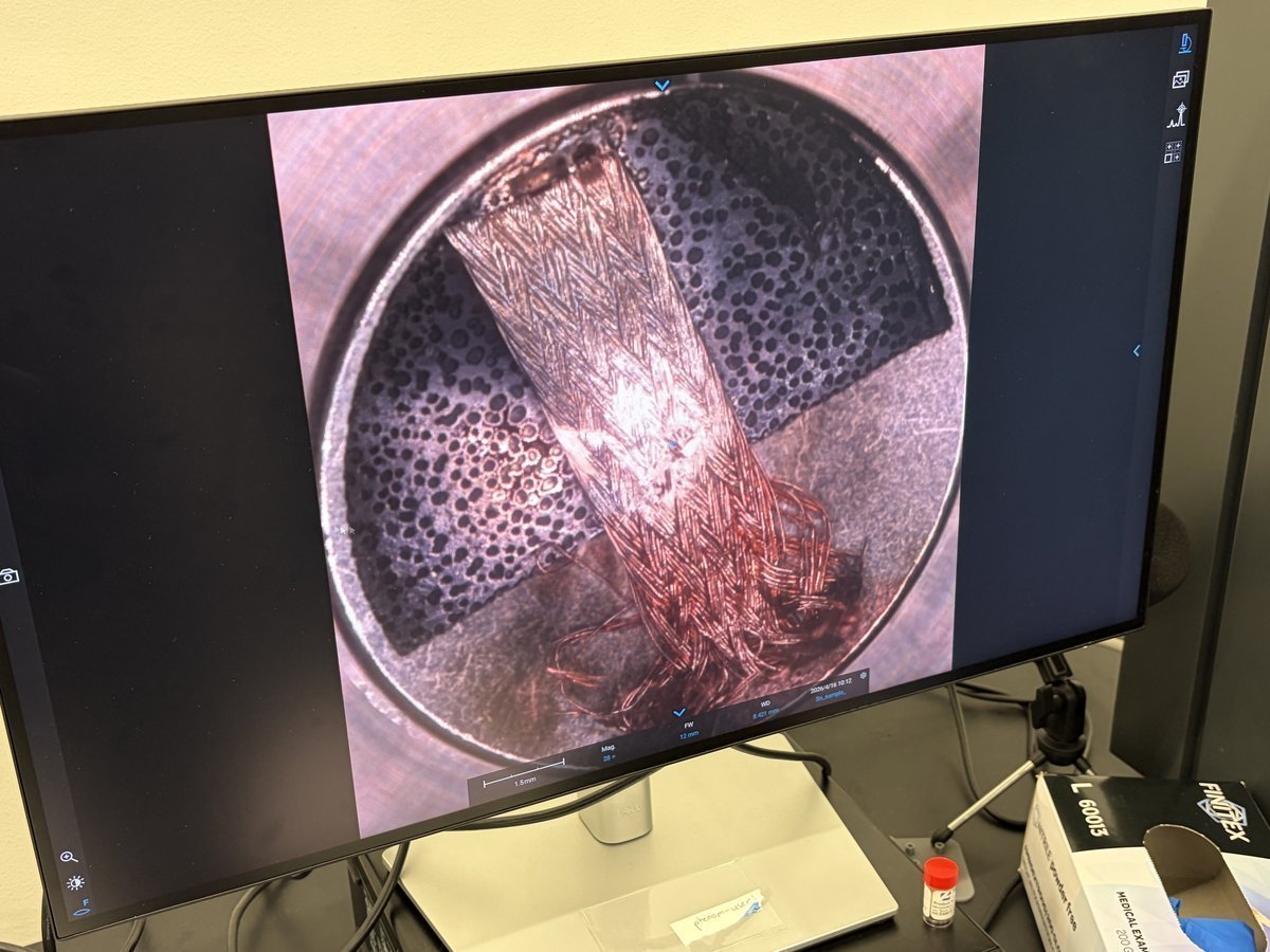
-
2.2 Set the save path and file naming
-
Configure acquisition settings
-
Click the gear icon in the left sidebar to open
Settings. -
Go to
Customize→Acquisition. Set theLabel(for example,Cu_sample) and theLocationpath (typicallyC:\Users\Phenom\Pictures\...\session N). -
The filename format will automatically include label, kV, magnification, detector, pressure, and date.
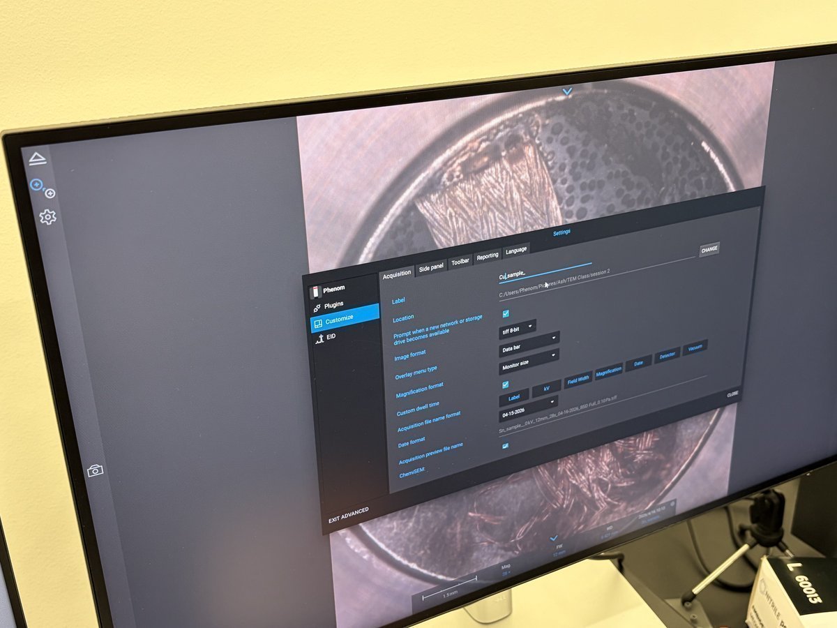
-
2.3 Move to SEM
-
Transfer sample to the electron beam
-
In the left sidebar, hover to reveal the
Move to SEMbutton. Click it to transfer the sample from the optical camera to the SEM beam.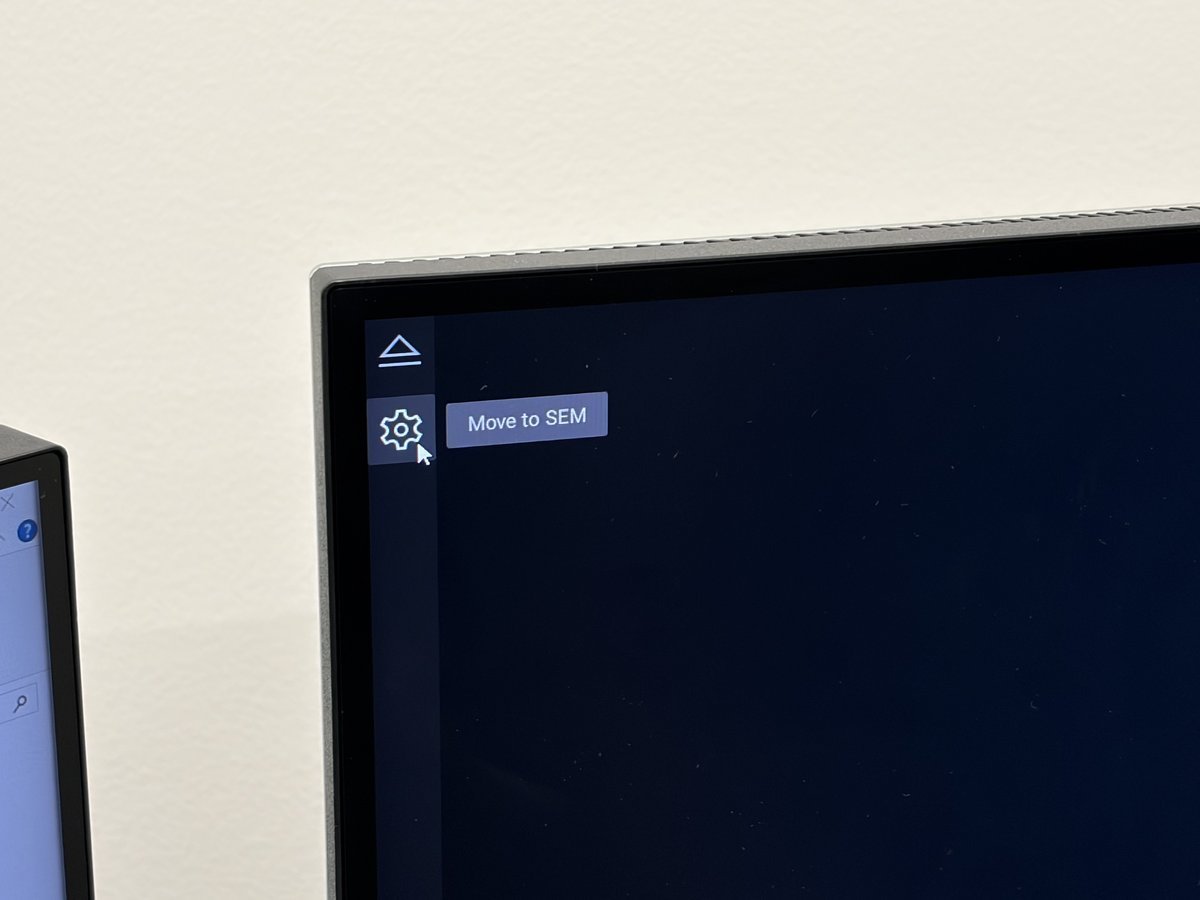
-
A progress indicator appears showing
Moving to SEM. This takes about 15 seconds.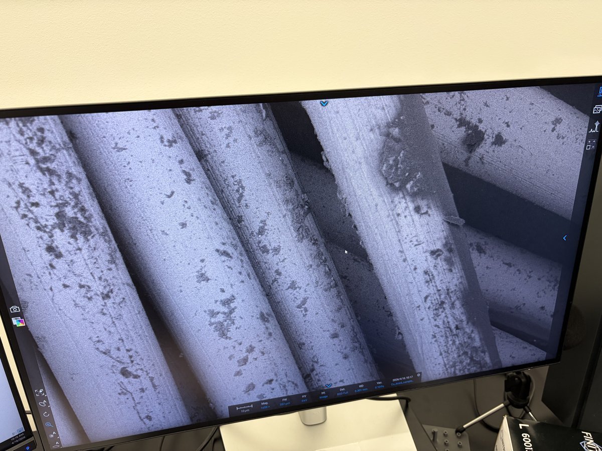
-
Set the accelerating voltage to a starting value (5 kV is a safe default for most samples).
NOTE: Higher kV (20 kV) gives better signal from BSE but more beam penetration. Lower kV (5 kV) is better for surface imaging and beam-sensitive samples.
-
Part 3: Imaging and tuning
3.1 Find an intermediate magnification
-
Navigate the sample
-
Scroll the mouse wheel to zoom in and out. Find a magnification that feels “intermediate” for your features (usually 1,000x to 10,000x to start).
-
Drag on the image to translate the stage. Features come into view as the stage moves.
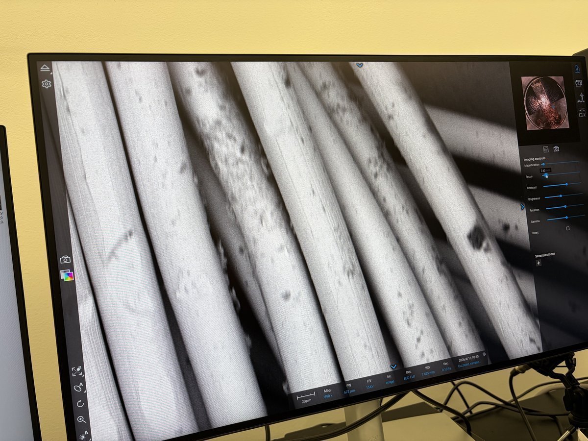
The right panel shows
Imaging controls: magnification slider, focus, contrast, brightness, rotation, gamma, and an invert toggle. Most of these you adjust by the auto buttons, not manually.
-
3.2 Tune the beam (the three auto buttons)
The Phenom has three auto-tuning buttons in the lower left corner. Use them in order every time you change kV, change detector, or move to a new region.
TODO for me to investigate: when to use auto vs. manual? The auto buttons handle most cases, but there are specific situations where you need to override them manually. Figure out:
- When does
Autofocusfail and require manual focus? (e.g., low-contrast regions, very flat samples)- When is manual stigmator adjustment better than
Autostigmate? (e.g., atomic-resolution tuning, asymmetric features)- When do you turn off
autoCBand set contrast/brightness manually? (e.g., comparing images across pressures, where the PDF says “leave autoCB alone” during the pressure series)- How does automatic scanning (tile series auto-positioning, auto-focus per tile) behave and when does it need manual correction? This is a known weak area to investigate in future sessions.
-
Run autofocus, autoCB, autostigmate
-
Click
Autofocusfirst. The system wobbles focus and settles on the sharpest value. -
Click
Auto contrast-brightness(autoCB). This normalizes the detector signal to fill the histogram. -
Click
Autostigmate. This corrects beam astigmatism (round beam shape).NOTE: Every time you change kV, rerun all three. When you only change detectors, autoCB is usually enough.
-
3.3 Acquire an image
-
Save an image
-
Set the
Scan sizeandDwell timein the acquisition panel.1920x1080atMediumscan is a good default for quick imaging. -
Click the camera icon on the left sidebar to acquire. The system does a high-quality scan and saves the image to your path.
NOTE: Files are saved as
.tiffwith metadata (kV, magnification, detector, pressure, WD, date) embedded.
-
-
Review in the image viewer
-
Double-click a saved
.tiffin Windows Explorer to open it in the Phenom Image Viewer. The right panel shows all acquisition properties.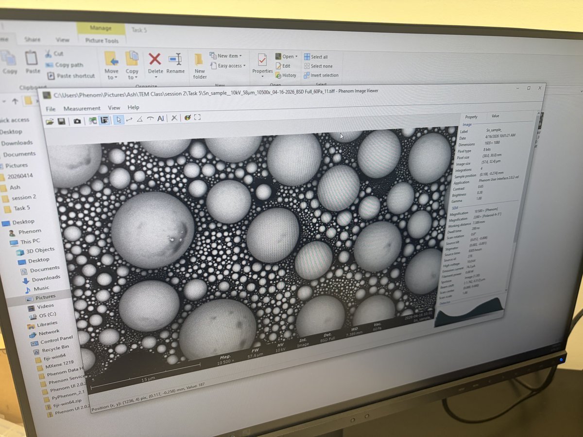
-
3.4 Detectors and modes
Once the sample is loaded and you are in SEM mode, open the top menu options panel to pick your accelerating voltage, beam intensity, detector, vacuum, averaging, scan size, and dwell time. These are all the settings you will touch during a session.
The Phenom Pharos supports multiple imaging modes. Switch between them from the Detector row in the settings panel.
| Mode | What it shows | When to use |
|---|---|---|
BSD Full | Backscattered electrons, all angles | Atomic number contrast (Z-contrast), compositional differences |
BSD Top | Backscattered, only top segment | Surface topography with Z-contrast |
SED | Secondary electrons | Fine surface topography. Not available at high pressure. |
4A+BSD+SED | Combined | Composite image |
Pressure affects which detectors are usable:
| Pressure | Use case |
|---|---|
| Low (0.1 Pa) | Best resolution. SED available. Default for most samples. |
| Medium (10 Pa) | Reduces charging on insulating samples. |
| High (60 Pa) | Use for heavily charging samples. SED not usable at this pressure. |
Part 4: Maps software for large-area tiles (Optional)
Warning
Part 4 is a placeholder. The Maps software is powerful but deserves its own dedicated tutorial: project templates, tile stitching, auto-focus per tile, rotation alignment, stitched navigation, high-resolution drill-in, and handling of sparse samples. The notes below are a sketch from a single session.
TODO: Write a full Maps walkthrough after more hands-on practice. Cover: template setup, optical → SEM transfer for tile planning, auto-focus behavior across tiles, rotation to match feature direction, nested high-resolution tile series, file organization of large datasets.
For mapping large areas (for example, a whole copper braid or the full width of a grid), switch to the Maps software for tile acquisition and stitching.
4.1 Open Maps and set up a tile series
-
Switch to Maps
- Press the Windows key on the keyboard to minimize the Phenom software.
- Launch
Maps(Thermo Scientific). - Create a new project. Set a template (Factory Template is fine for a first pass).
-
Configure the tile series
-
In
Maps, set the number of tiles (for example, 3x3 or 4x4 to start). -
Set the tile HFW (horizontal field width), resolution (for example, 1920x1080), averaging, contrast, and brightness.
-
Position and rotate the tile grid over the region of interest on your optical overview.
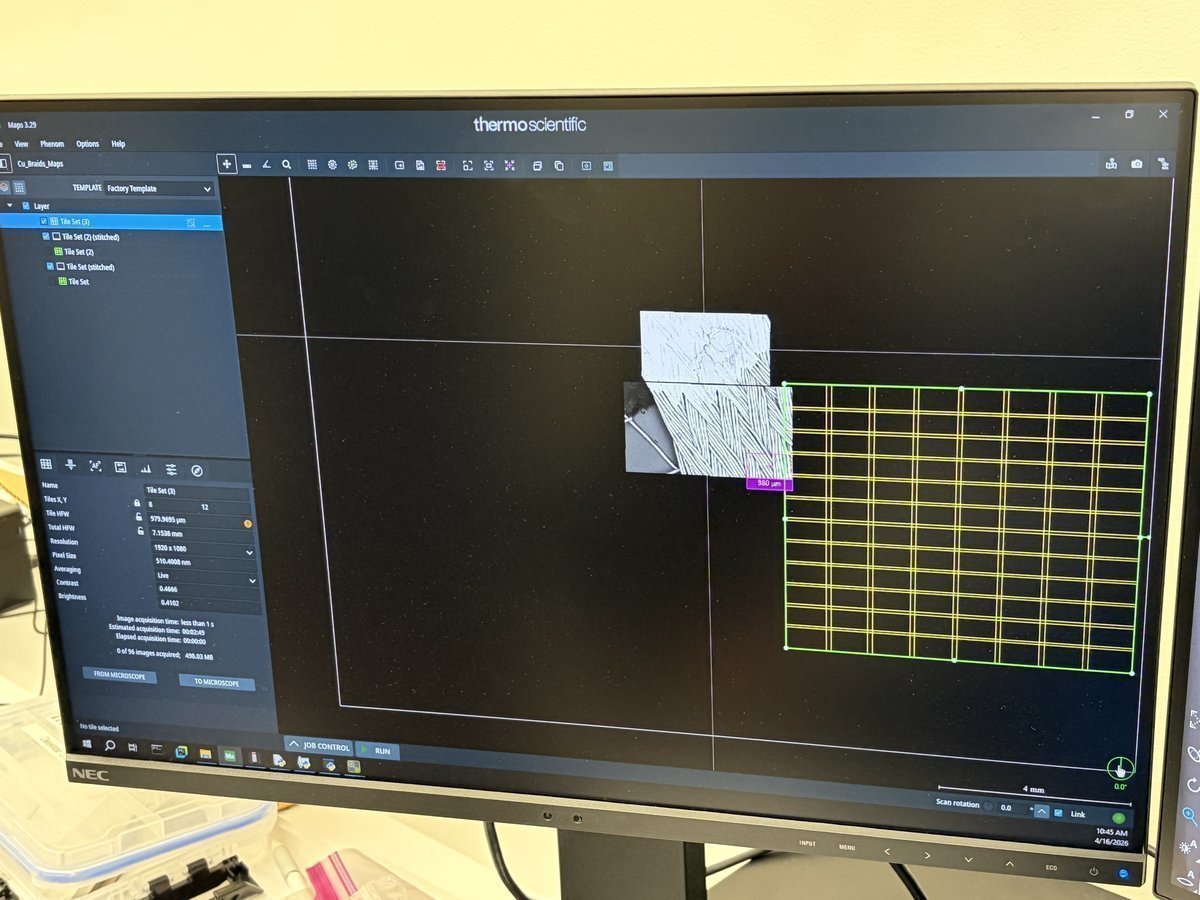
-
4.2 Run the tile series
-
Acquire tiles
-
Click
RUNat the bottom.Mapstakes over the microscope and acquires each tile. -
A progress bar shows remaining time (for example, “4 of 16 images acquired, 1.43 GB”).
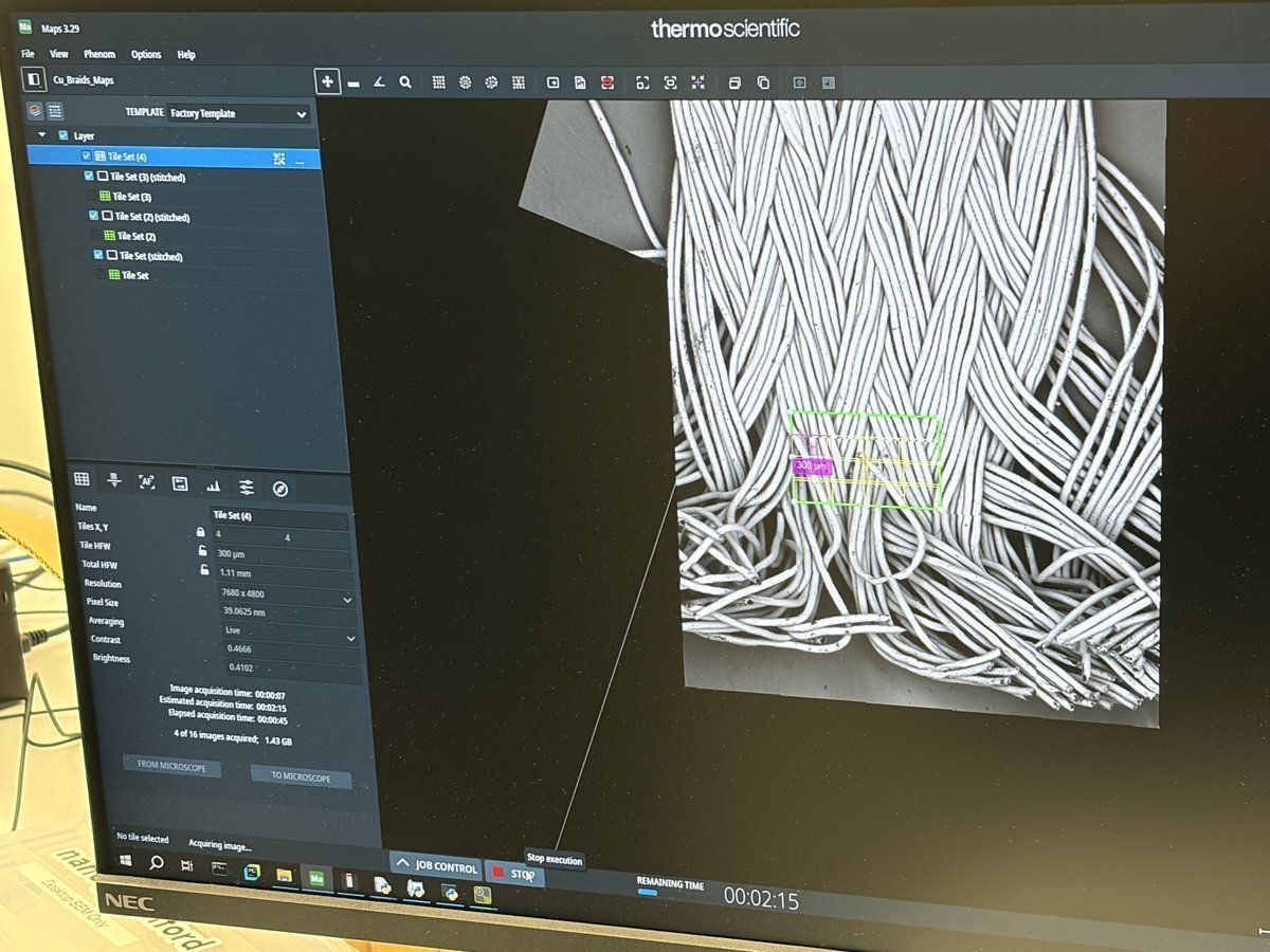
-
After all tiles are acquired,
Mapsautomatically stitches them into a single stitched layer.
-
-
Drill into a region
- Use the stitched map to navigate to an area of interest.
- Set a smaller, higher-resolution tile series on top of the first to map that area at finer detail. Keep the second series small to avoid a long acquisition (aim for 3-5 min).
Part 5: STEM mode (Optional)
STEM imaging requires swapping to the STEM holder, which has a segmented transmission detector built into the stub. The holder takes a standard 3 mm TEM grid on top.
5.1 Swap to the STEM holder
-
Retrieve the STEM holder
-
Unload the current sample (see Part 6).
-
Take the STEM holder out of its storage case. The STEM holder has a circular transmission detector window in the center of the stub.
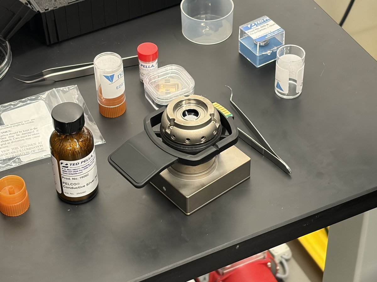
NOTE: The STEM holder itself contains the BF/DF/HAADF segmented detectors. The grid sits on top of the detector, and transmitted electrons pass through the grid and hit the segmented detector below.
-
5.2 Load a TEM grid
-
Place the grid, blue side down
-
Use fine-tip tweezers to pick up the TEM grid by the edge.
-
Lower the grid into the holder slot with the blue side facing down. The sample side faces up toward the beam.
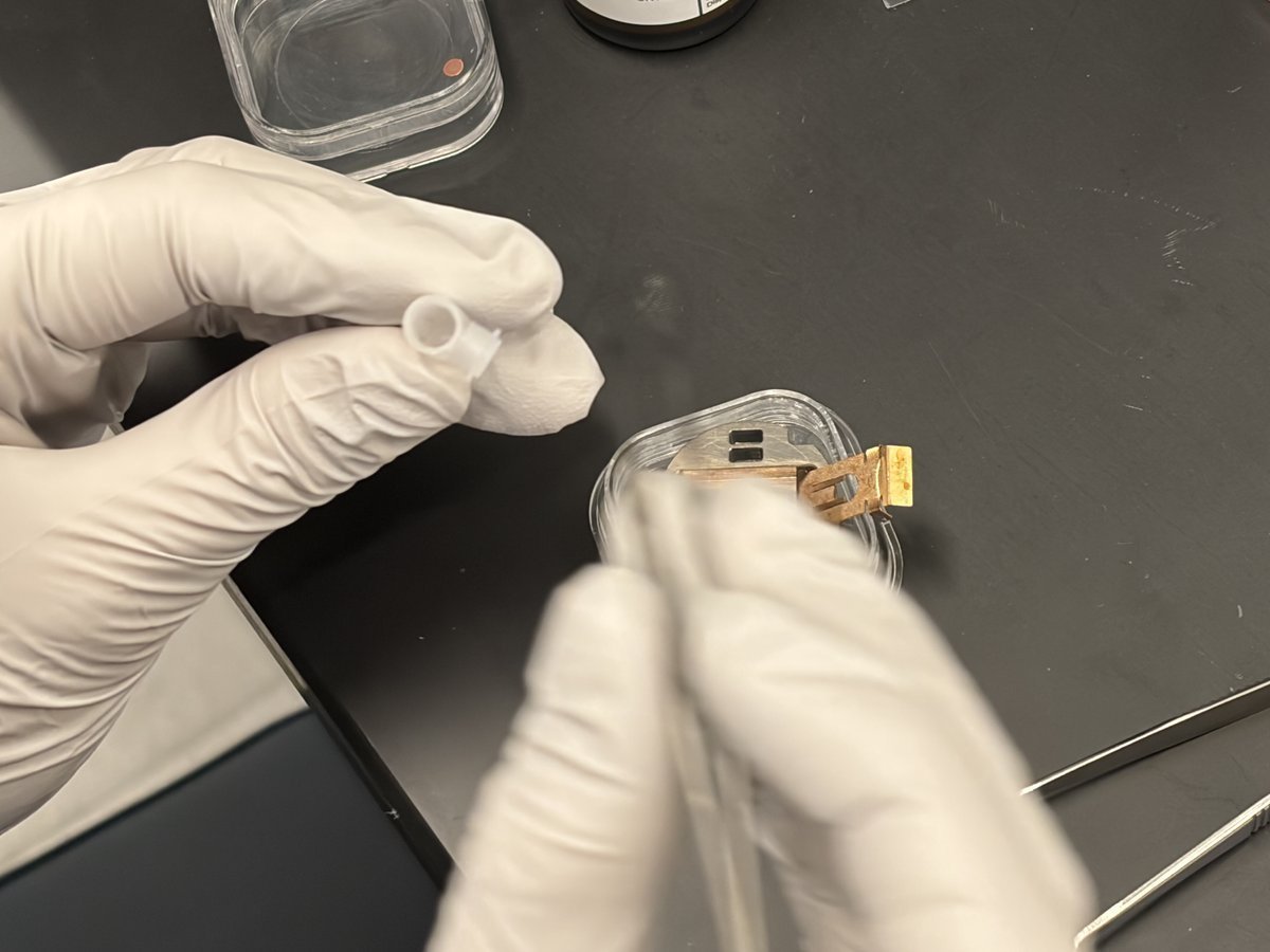
-
Seat the grid flat so it does not shift during pumping.
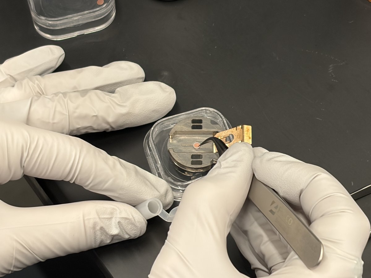
-
-
Add the washer and close
-
Place the washer on top of the grid to secure it in the holder.
-
Close the retaining cap.
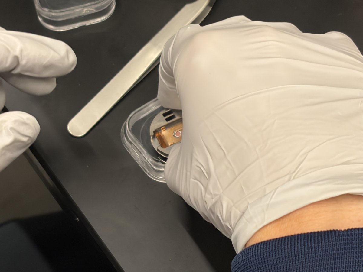
-
5.3 Insert the STEM holder
-
Load into the Phenom
-
Place the STEM holder into the drawer the same way as a regular stub.
-
Close the drawer. The green LED on the inside confirms the holder is seated correctly.
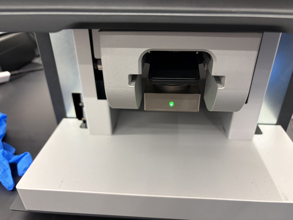
-
5.4 Switch to STEM imaging
-
Enter BF STEM mode
- Once pumping completes and the sample moves to the SEM, the system defaults to BSE Full. Switch to 5 kV.
- Zoom into one of the dark grid squares until the Cu grid bars are no longer visible.
- In the detector selector, switch to
BF STEMmode. - Run autoCB, autofocus, and autostigmate in that order.
-
Compare detectors
-
Cycle through
BF STEM,DF STEM, andHAADF STEMto compare contrast mechanisms on the same region. Run autoCB each time you switch detector.When to use each STEM mode:
BF STEM: absorption contrast, shows thickness variations. Good for polymers, biological samples.DF STEM: diffraction contrast, shows crystalline grains.HAADF STEM: Z-contrast, heavier atoms appear brighter. Good for nanoparticles.
-
Part 6: End session
-
Save and back up images
-
Verify all images are saved to your session folder. Check the filename format includes sample label, kV, magnification, detector, pressure, and date so you can identify them later.
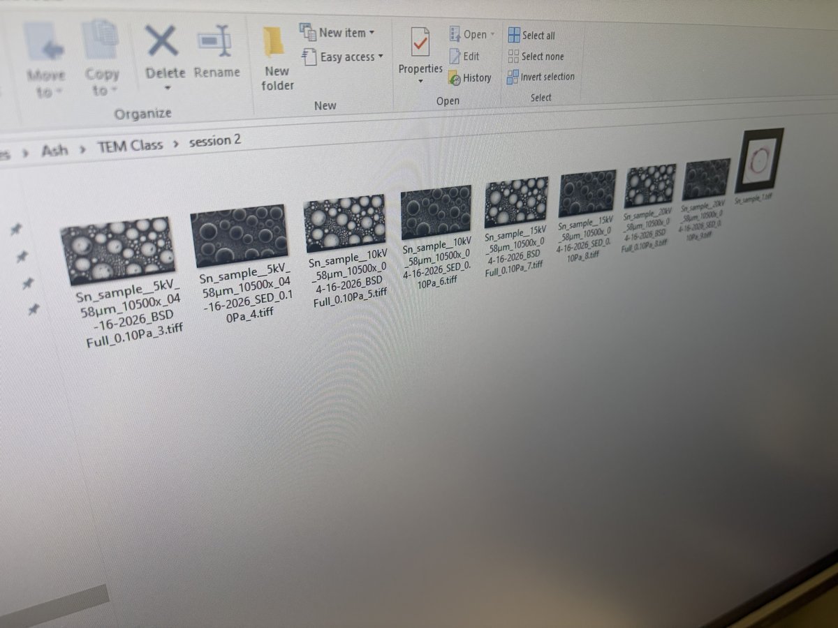
-
Copy the folder to external storage or a network drive before leaving.
-
-
Unload the sample
- In the software, click the eject icon (triangle in the left sidebar) to vent the chamber. Wait for the vent cycle to complete.
- Open the drawer and remove the stub or STEM holder.pressure.
-
Return to storage
- Return the stub puck holder and STEM holder to their storage locations.
- Close the drawer empty to protect the chamber.
-
Hand off
- Log the session in the booking/logbook as required by lab rules.
- Wipe down the bench and return gloves/tweezers to their locations.
Part 7: Lab observations from the Theme 1C session (MATSCI 322)
This section captures the data and comparisons that came out of the Theme 1C class lab from the Stanford MATSCI 322 TEM Lab (taught by Andrew Barnum, Pinaki Mukherjee, and Ash) on the same Phenom Pharos: three full acquisition tables (Cu braid kV by detector, Cu braid kV by pressure, STEM cross-grating kV by detector) followed by discussion of BSE vs SED contrast, the kV impact, the pressure series, and the STEM transmission contrast.
Acquisition Table 1: Cu braid, kV by detector (low pressure)
Acquired at low chamber pressure (~0.10 Pa). Each kV was retuned with autofocus / autoCB / autostigmate, so working distance and magnification drift slightly between columns; the actual values are listed in the captions.
| 5 kV | 10 kV | 15 kV | 20 kV | |
|---|---|---|---|---|
| BSE Full | 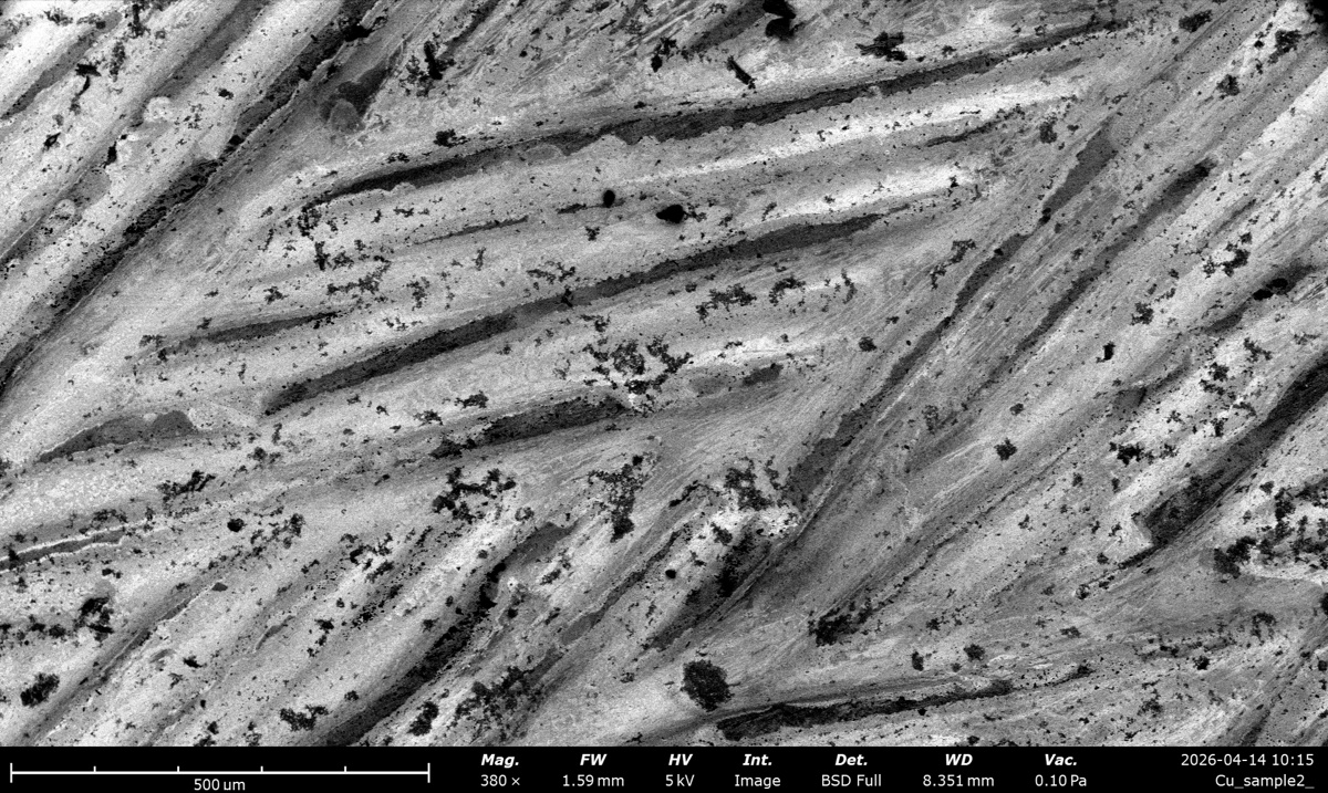 380×, WD 1590 µm |
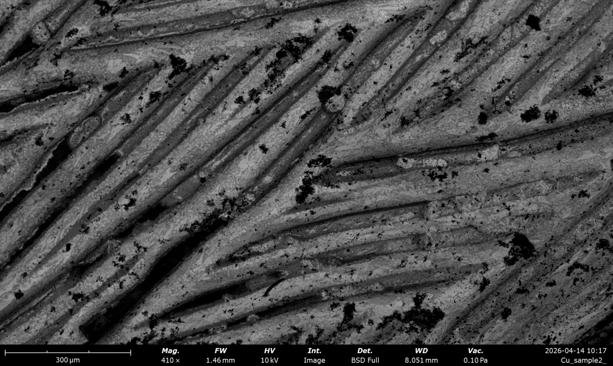 410×, WD 1465 µm |
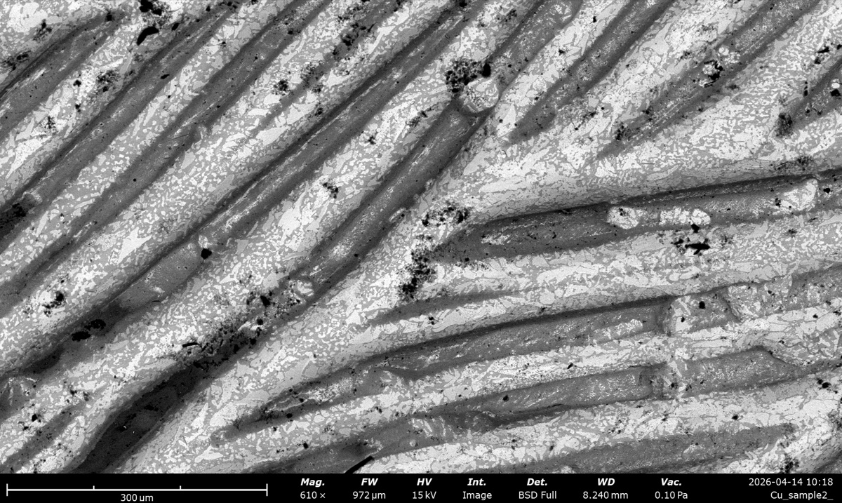 610×, WD 972 µm |
 810×, WD 733 µm |
| SED | 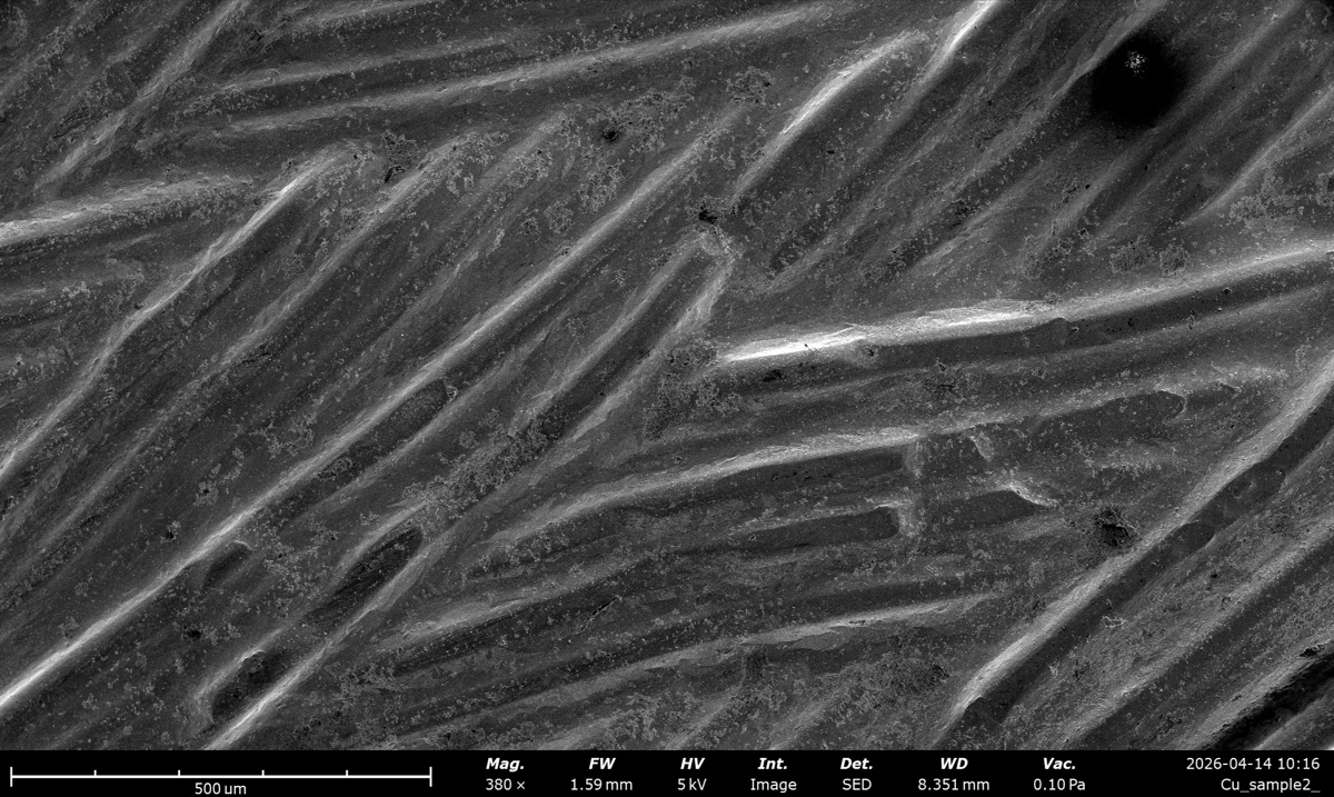 380×, WD 1590 µm |
 410×, WD 1465 µm |
 610×, WD 972 µm |
 810×, WD 733 µm |
Acquisition Table 2: Cu braid, kV by pressure (BSE Full at 810x)
Pressure series held at fixed magnification (810×) and BSE Full detector. The achievable chamber pressure depends on kV, so the qualitative tiers (Low / Medium / High) correspond to different absolute pressures across columns; actual values are listed in each cell. kV was retuned between columns; autoCB was left alone within a column.
| 5 kV | 10 kV | 15 kV | 20 kV | |
|---|---|---|---|---|
| Low (~0.1 Pa) |  0.10 Pa |
 0.13 Pa |
 0.81 Pa |
 0.35 Pa |
| Medium (~3 to 5 Pa) |  4.0 Pa |
 5.0 Pa |
 2.8 Pa |
 4.5 Pa |
| High (~20 to 33 Pa) |  27 Pa |
 24 Pa |
 33 Pa |
 20 Pa |
Acquisition Table 3: STEM cross-grating with latex spheres, kV by detector
High-magnification series (16,000× at 5 kV, 17,500× elsewhere) at low pressure (0.10 Pa). All five detectors collected at each kV. The 12 mm / 28× overview shot used for navigation is shown below the table.
| 5 kV | 10 kV | 15 kV | 20 kV | |
|---|---|---|---|---|
| BF STEM | 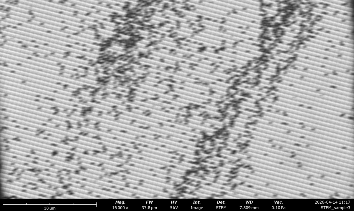 |
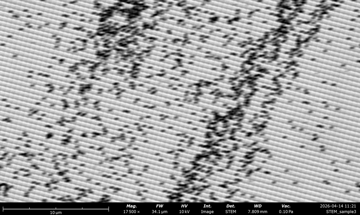 |
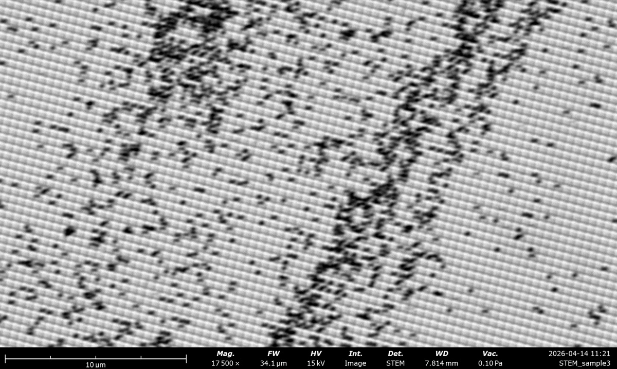 |
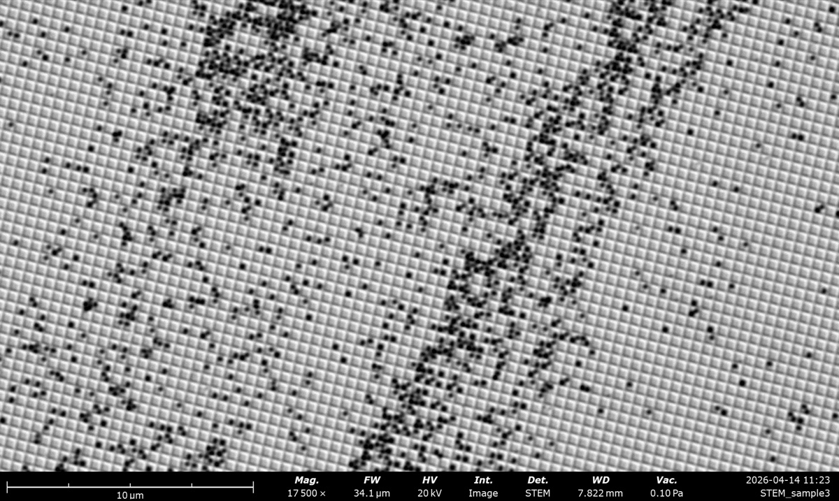 |
| DF STEM | 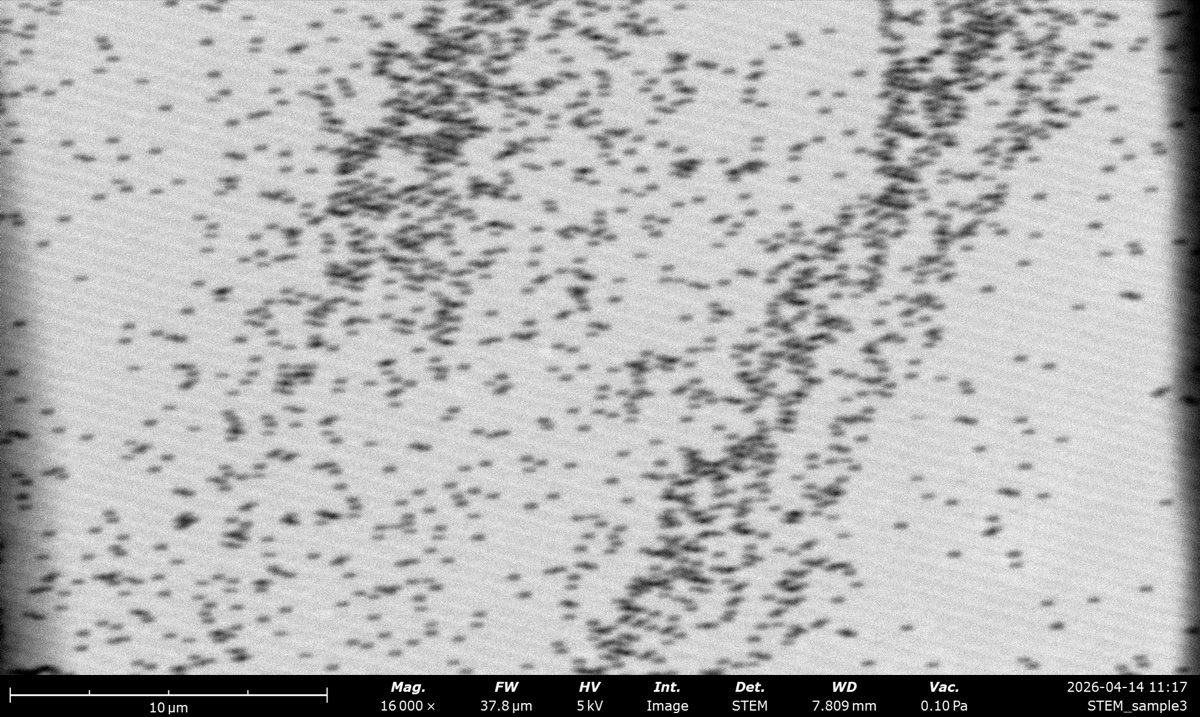 |
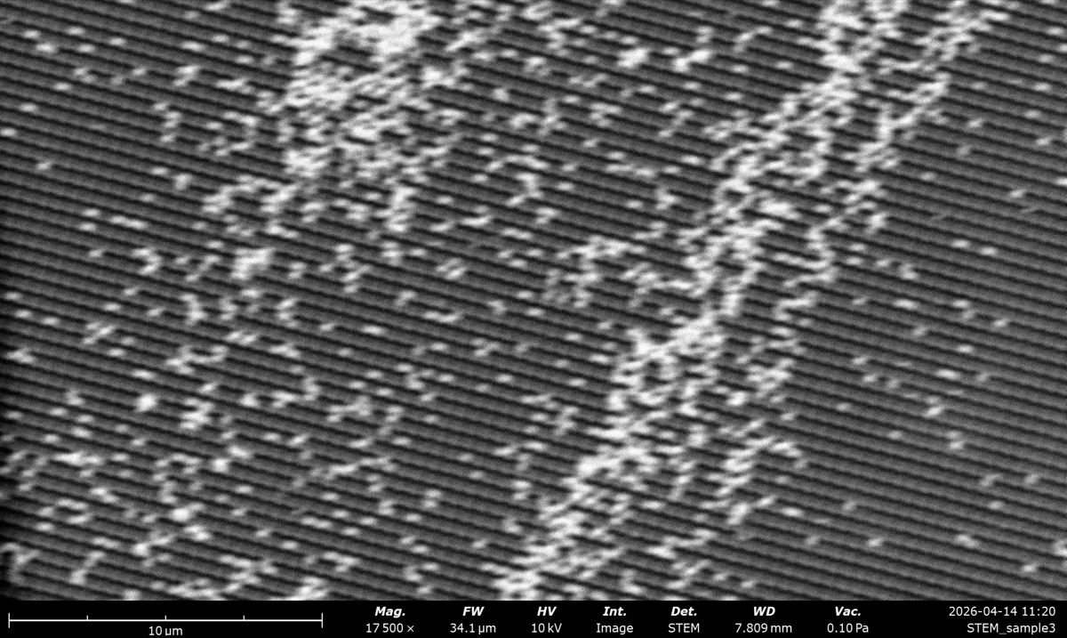 |
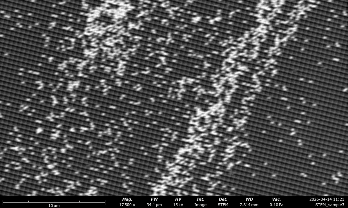 |
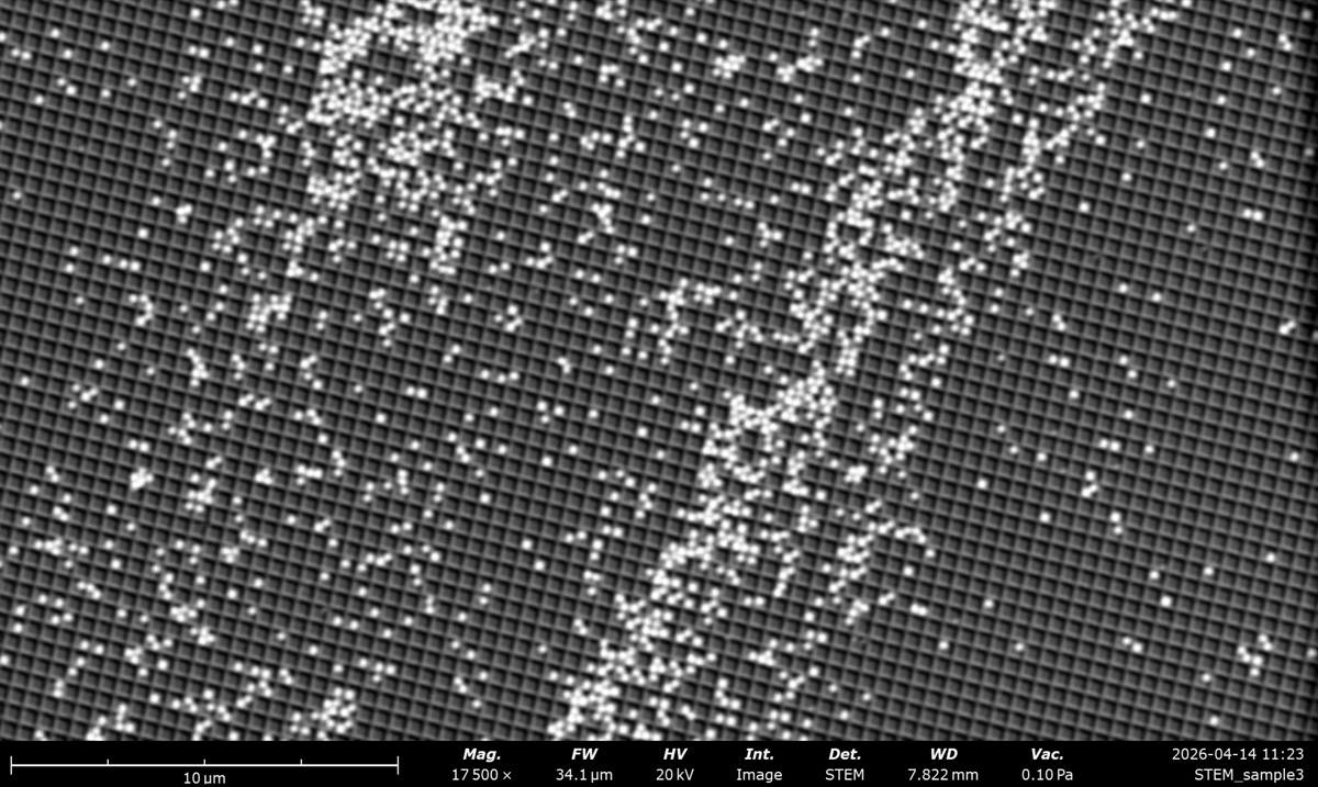 |
| HAADF STEM |  |
 |
 |
 |
| BSE Full |  |
 |
 |
 |
| SED | 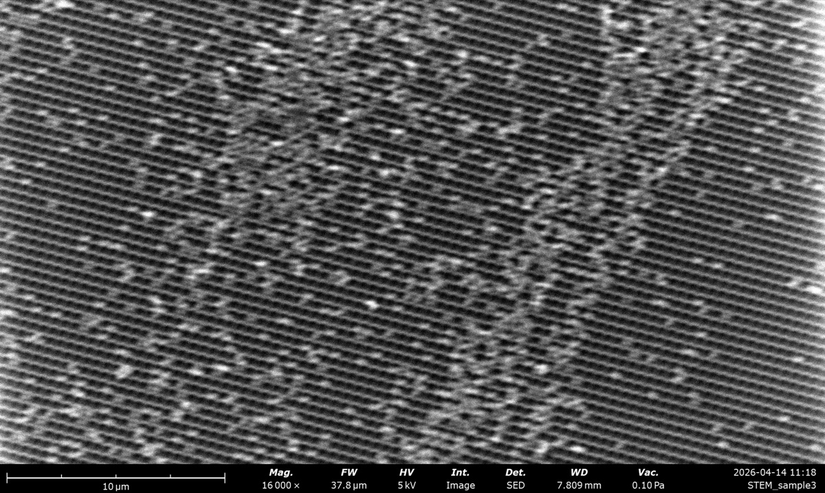 |
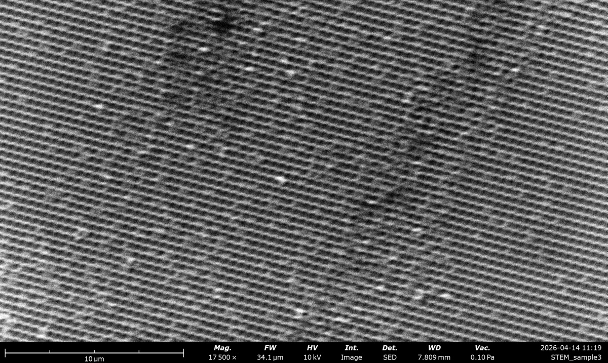 |
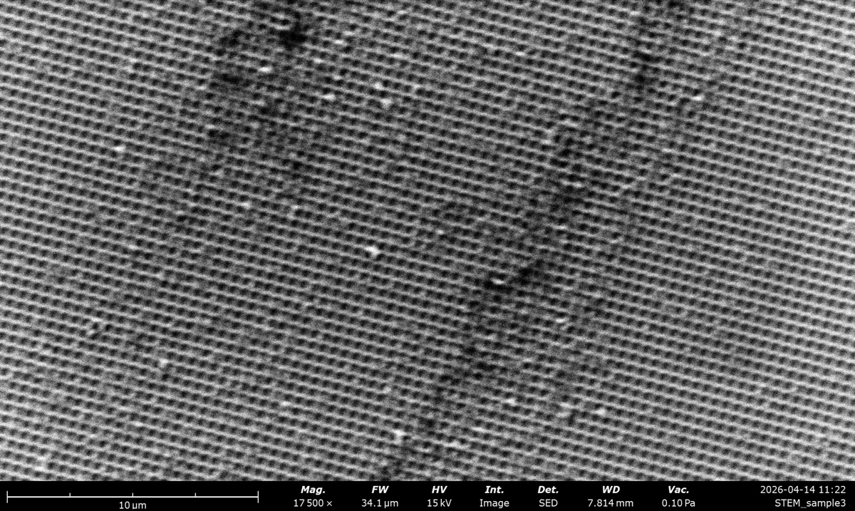 |
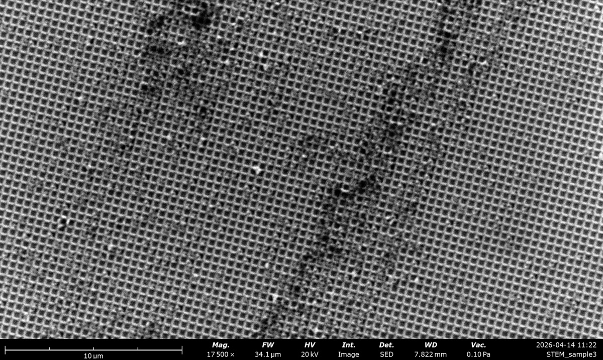 |
Overview shot (used for navigation)
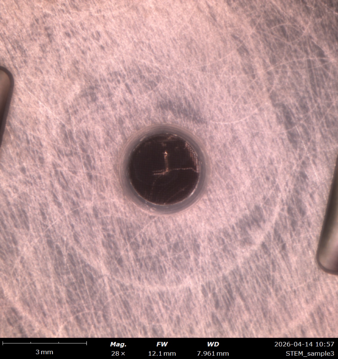
28×, WD 12 mm, 0.10 Pa: low-magnification overview used to locate a dark grid square before zooming in and switching to BF STEM mode.
Why BSE and SED look different
SED collects low-energy secondary electrons from the top ~5 nm and shows surface topography. BSE collects high-energy backscattered electrons from deeper in the interaction volume and shows composition (heavier elements brighter). At 20 kV on an ion-polished Cu braid, the contrast difference is striking:
20 kV BSE Full: composition contrast (heavier elements brighter) |
20 kV SED: surface topography (scratches and edges) |
kV impact, and the kV regime where BSE looks like SED
Higher kV grows the interaction volume, so BSE picks up more Z contrast but blurs surface detail, and SED loses surface fidelity to “SE2/SE3” electrons generated by exiting backscatter. At very low kV (~1 to 3 kV) the interaction volume is shallow enough that BSE and SED sample essentially the same near-surface region and the two images converge.
5 kV BSE Full: shallow pear, surface bleeds into BSE |
5 kV SED: surface topography, close to the 5 kV BSE image |
Pressure: contrast washout, autoCB, and why SED fails at high pressure
Gas in the chamber scatters the primary beam into a diffuse “skirt” that raises the background and washes out contrast. autoCB rescales the histogram but cannot bring back lost spatial detail. SED fails at high pressure because the +10 kV grid would arc, and the low-energy electrons get absorbed by the gas before reaching the detector. High-pressure imaging therefore relies on BSE or a dedicated GSED.
0.10 Pa: sharp, full contrast |
4.0 Pa: contrast softening |
27 Pa: washed out, fine features lost |
Why STEM is clearer than BSE/SED for the latex spheres
STEM uses transmitted electrons, so the full thickness of each sphere contributes to the signal. Low-Z thin objects barely register in BSE or SED but pop in STEM via mass-thickness contrast (BF darkens, DF/HAADF brightens). Low kV (5 kV) gives strong contrast but noisier images; high kV gives weaker contrast but sharper images.
5 kV BF STEM: spheres dark on bright background |
5 kV BSE Full: low-Z spheres barely visible |
5 kV SED: flat, no surface to light up |
Acknowledgments
Thank you to TA Ash for running the Phenom Pharos lab walkthrough on Apr 16, 2026. Photos captured during the session by @bobleesj.
Changelog
- May 11, 2026 - Added Part 7 (lab observations from the Theme 1C session) covering BSE vs SED, kV impact, pressure series, and STEM transmission contrast on the latex sphere cross grating, with comparison thumbnails by @bobleesj.
- Apr 16, 2026 - Initial rough draft from Ash TA session and Theme 1C lab PDF by @bobleesj
Talos bright-field and dark-field imaging
Caution
VERY ROUGH DRAFT. Notes from a Stanford MATSCI 322 TEM Lab session taught by Andrew Barnum, Pinaki Mukherjee, and Ash. This guide is being expanded and refined as @bobleesj uses the Talos in future sessions. Steps and screenshots still need verification against the live instrument.
TODO: Add stage navigation, eucentric height alignment, selected-area aperture insertion, condenser aperture changes, dose-on-sample calibration, and end-of-session shutdown.
This guide covers the operational steps for bright-field (BF) and dark-field (DF) imaging on the Talos TEM, captured during a class session in April 2026. It also includes a reference example of how under- and over-focused images appear on the FluCam, which is useful when interpreting defocus during alignment.
Acronyms:
BF: bright fieldDF: dark fieldTEM: transmission electron microscopeSTEM: scanning transmission electron microscopeFFT: fast Fourier transformVelox: Thermo Fisher acquisition software for the TalosFluCam/SmartCam: fluorescent screen camera (used for alignment)Ceta: high-resolution CMOS camera mounted below the phosphor screenmulXY: multi-function X/Y knobs on the hand panel
Overview
| Phase | What it covers | Time |
|---|---|---|
| Part 1: Startup and orientation | System settle, identify legacy hardware, vacuum check | 5 min |
| Part 2: Open Velox and select a camera | Launch Velox, choose FluCam or Ceta | 2 min |
| Part 3: Configure acquisition parameters | Frame size, frame combining, shutter, recording mode | 3 min |
| Part 4: Bright-field imaging | Open valves, navigate, set illumination, annotate | varies |
| Part 5: Dark-field imaging | Beam tilt, dark-field toggle, BF/DF comparison | 10 min |
Part 1: Startup and orientation
1.1 Allow the system to settle
-
Wait for the column to reach steady state
- Wait 2 to 3 minutes after powering up the Talos console before interacting with the column.
- Confirm the vacuum and high-tension subsystems have stabilized.
1.2 Locate the legacy hardware buttons
-
Identify the legacy controls on the console
-
Identify the legacy hardware buttons on the console. These exist because, before live FFT was available, focus had to be judged on the phosphor screen using the “Wobbler” feature, which modulates the beam to highlight the focused condition.
-
Use the live FFT in
Veloxfor routine focusing. The legacy controls remain functional as a backup.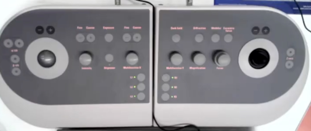
-
1.3 Check the vacuum overview
-
Confirm vacuum status
-
Open the Talos UI vacuum overview panel.
-
Confirm the column vacuum reads green before opening the column valves.
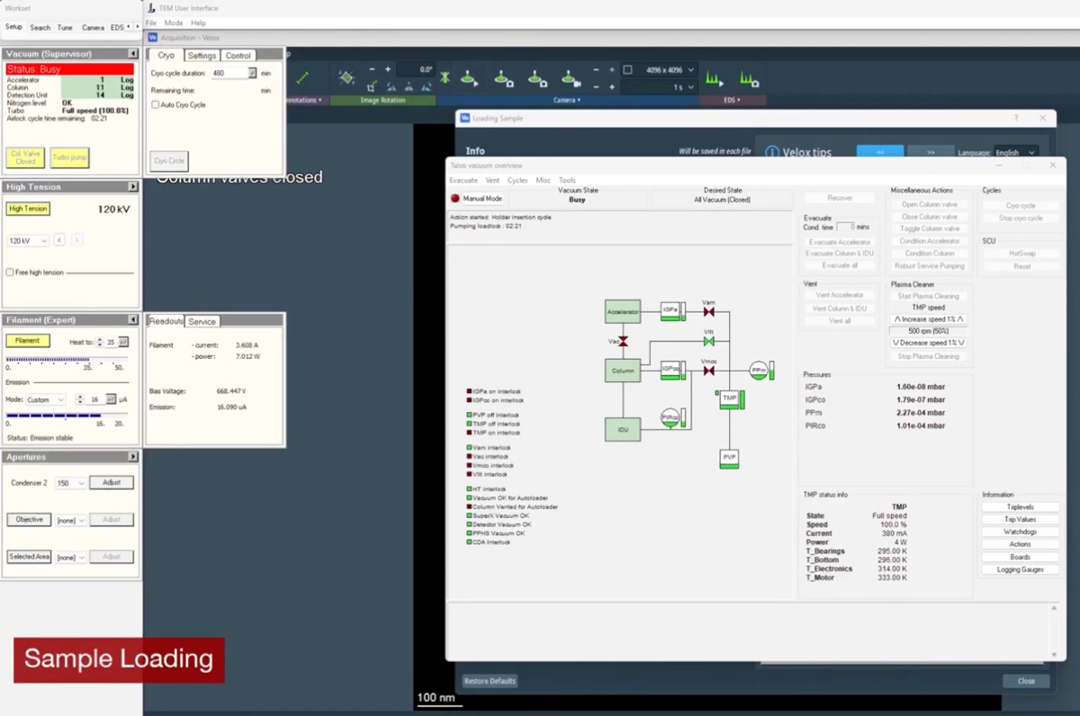
CRITICAL: Do not proceed if any vacuum gauge is yellow or red. Contact staff.
-
Part 2: Open Velox and select a camera
2.1 Launch Velox
-
Open the Velox acquisition software
-
Launch
Veloxfrom the desktop.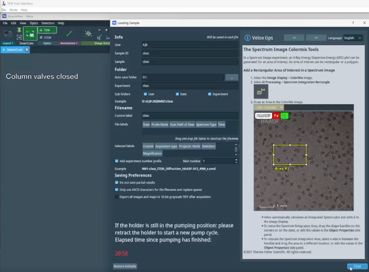
-
2.2 Select the FluCam for initial setup
-
Use the FluCam during alignment
- Select the
FluCam(also labeledSmartCamin some menus) for initial setup and alignment. The FluCam points at the phosphor screen rather than receiving the direct beam. - Use this camera for any operations that risk a high beam dose, since it protects the more expensive
CetaCMOS camera underneath.
- Select the
2.3 Switch to the Ceta camera for final acquisition
-
Switch to Ceta when alignment is satisfactory
-
Switch to the
Cetacamera once the alignment is complete and a high-resolution image is required.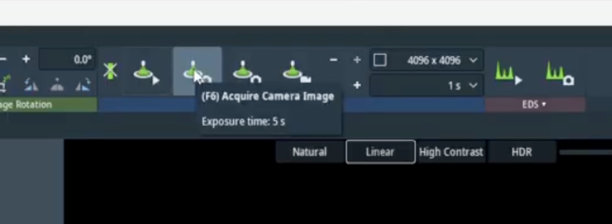
-
Part 3: Configure acquisition parameters
3.1 Open the acquisition presets
-
Open both acquisition presets
-
Open the two acquisition presets in
Velox. -
Update the parameters in each preset as needed during the session.
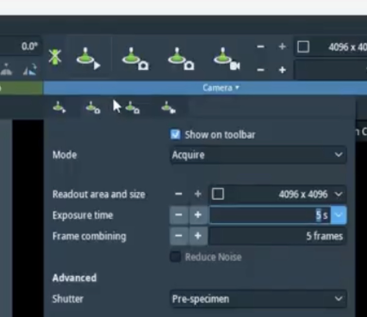
-
3.2 Set frame size and frame combining
-
Set 1024 by 1024 frames with 200 ms combining
-
Set the frame size to 1024 by 1024 pixels.
-
Set the frame combining to 200 ms. Frame combining averages multiple short exposures into a single output frame, which improves signal-to-noise without committing to one long exposure.
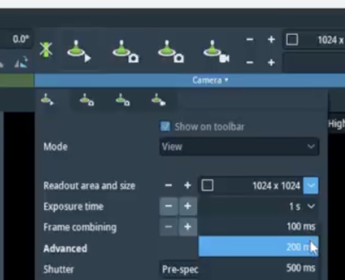
-
3.3 Choose the shutter
-
Pick pre-specimen or post-specimen shutter
-
Choose the pre-specimen shutter to block the beam before it reaches the sample. This protects beam-sensitive samples between exposures.
-
Choose the post-specimen shutter (a projection blanker) to block the beam after the sample. This controls exposure on the camera without changing illumination on the sample.
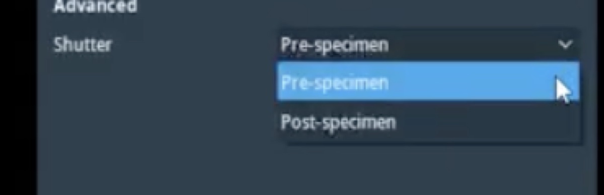
-
3.4 Choose the recording mode
-
Pick the recording mode that matches the experiment
-
Choose Auto Stop to record a fixed number of frames and then halt. This is the default for still imaging.
-
Choose Circular to keep the most recent N frames in a rolling memory buffer; pressing stop preserves whatever is in the buffer. This is useful for in-situ experiments where the moment of interest is unpredictable.
-
Choose Continuous to save every frame for the full duration of the recording.
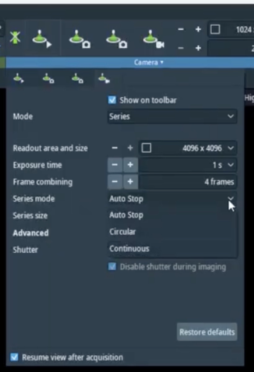
-
3.5 Open the column status bar
-
Show the column status bar during acquisition
-
Open the column status bar so the beam state, vacuum, and stage coordinates remain visible during acquisition.
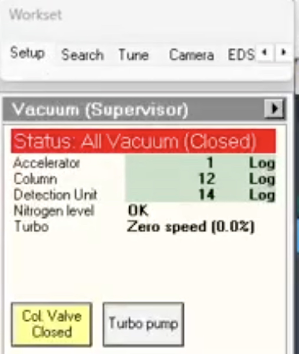
-
Part 4: Bright-field imaging
4.1 Open the column valves
-
Open the column valves once vacuum is green
-
Open the column valves from the Talos UI.
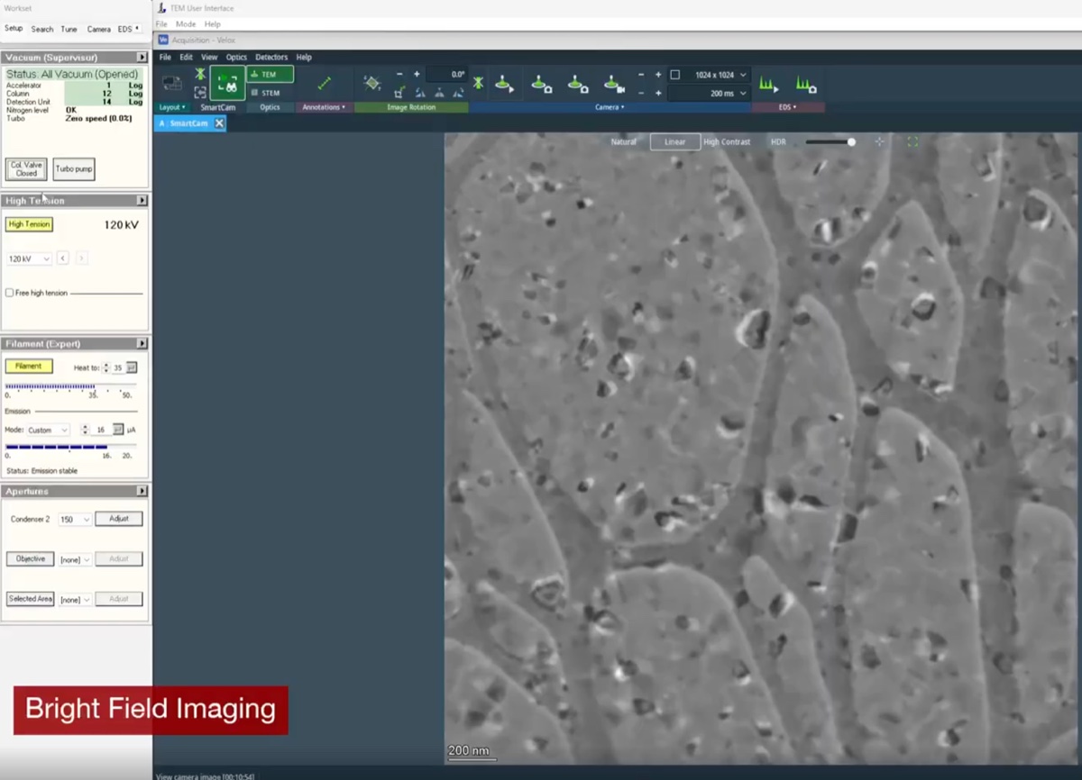
-
4.2 Drop to low magnification to find the feature of interest
-
Navigate at ~25x magnification
-
Drop the magnification to roughly 25x using the magnification knob.
-
Move the stage to a feature of interest using the trackball.
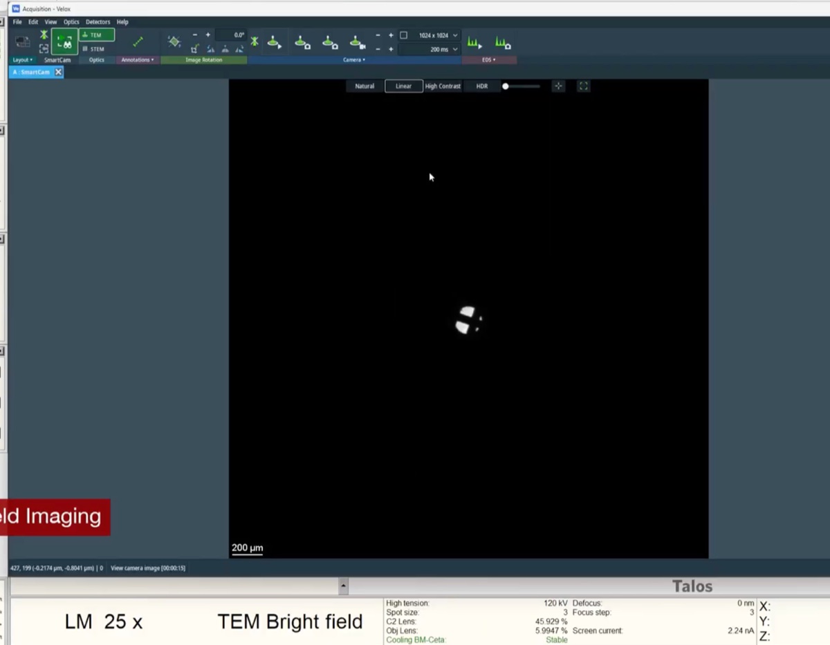
-
4.3 Set the illumination
-
Use the intensity knob to spread or condense the beam
- Turn the intensity knob until the illumination on the sample is uniform and the histogram fills the dynamic range without saturating.
4.4 Acquire and annotate
-
Acquire and annotate a bright-field image
-
Acquire an image with the chosen camera.
-
Use the
Veloxannotation tool to label features, mark positions, or add scale annotations.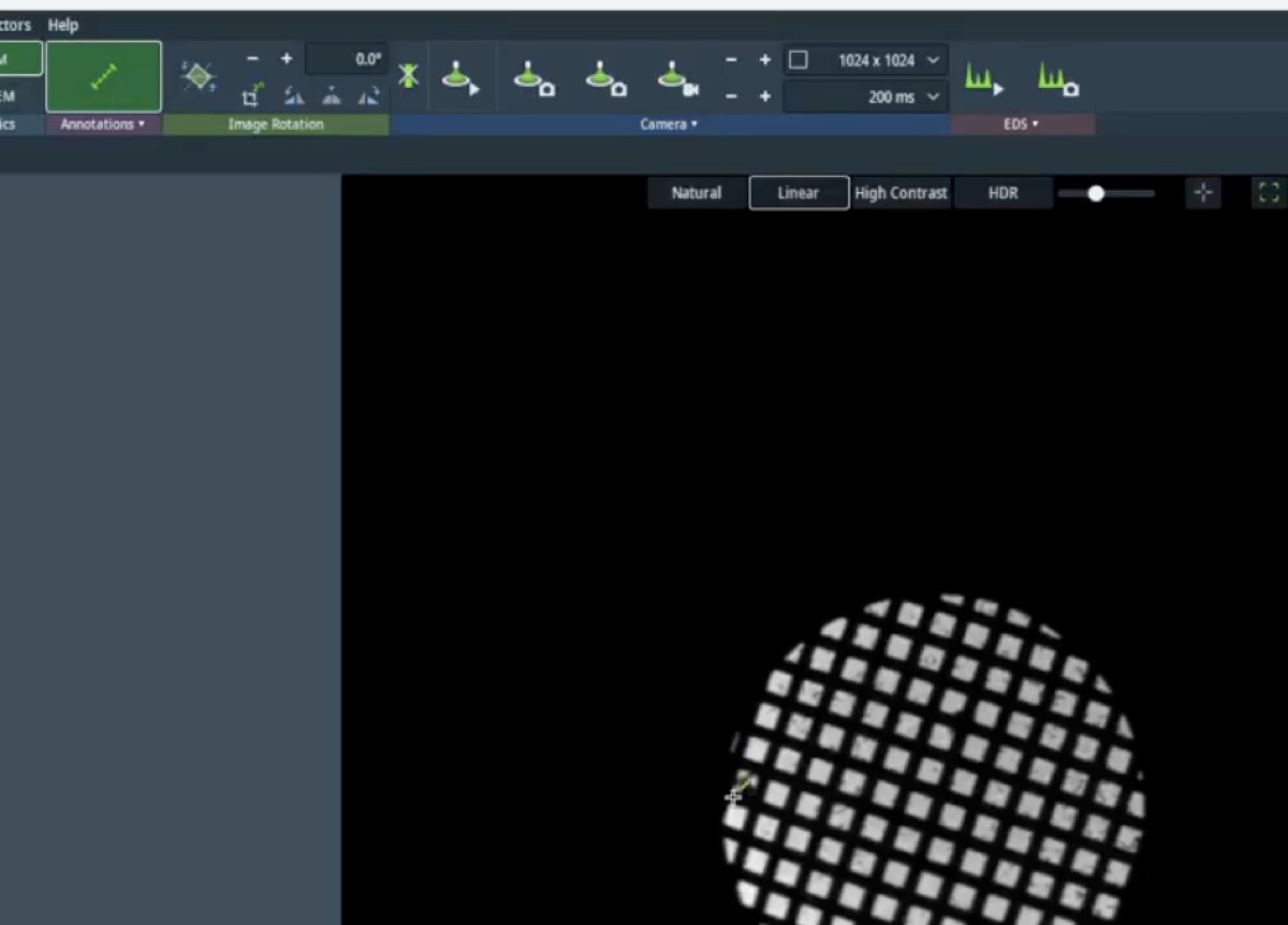
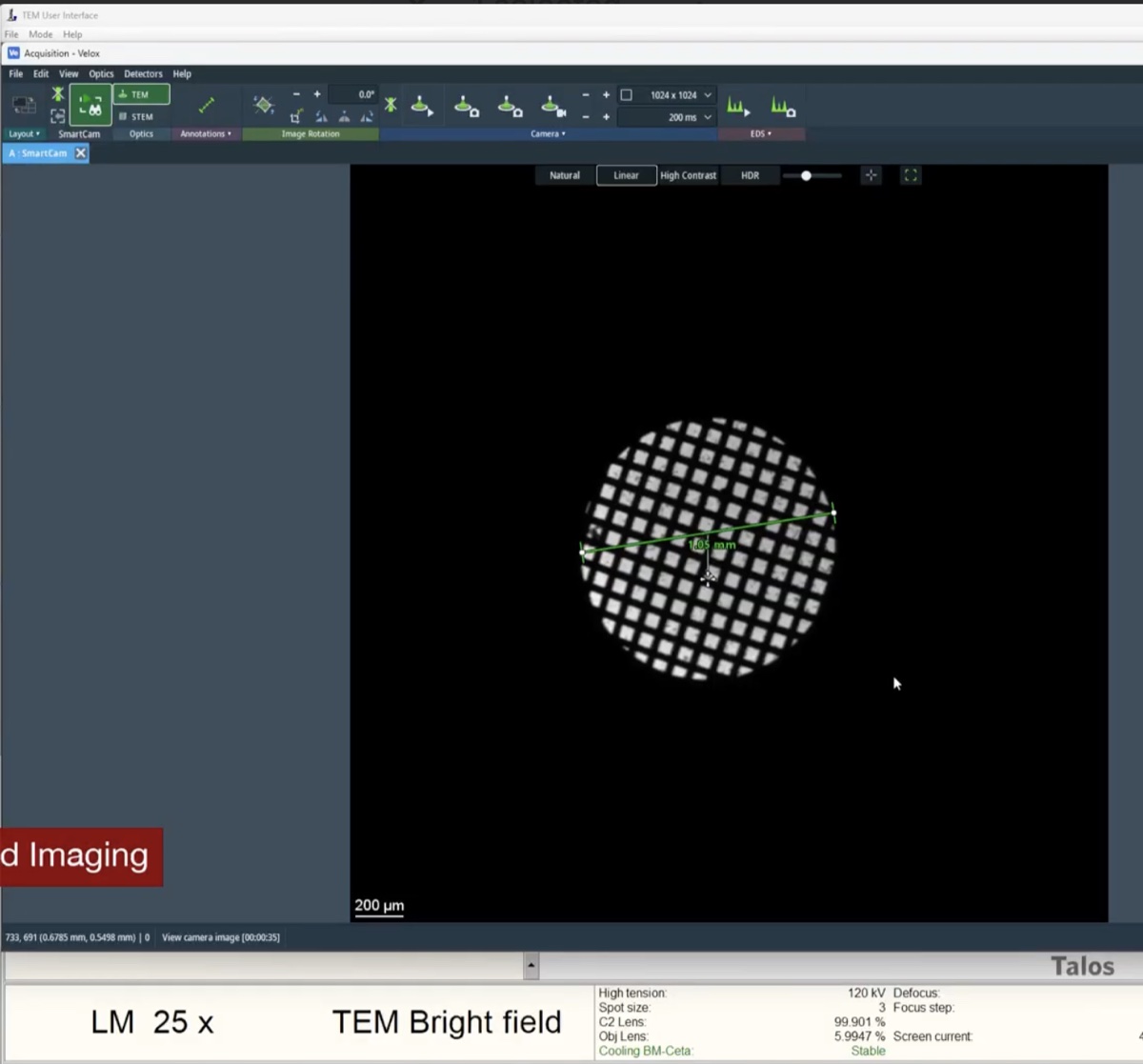
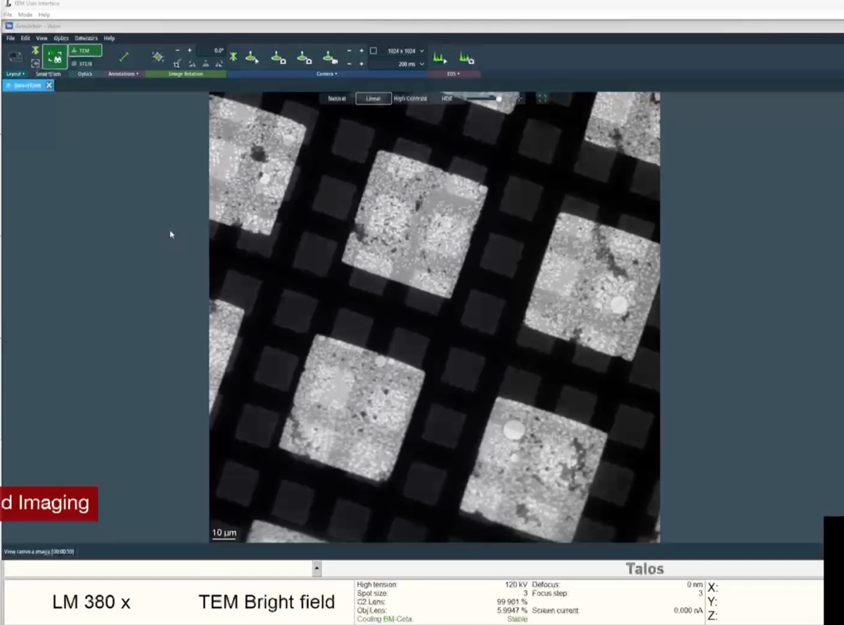
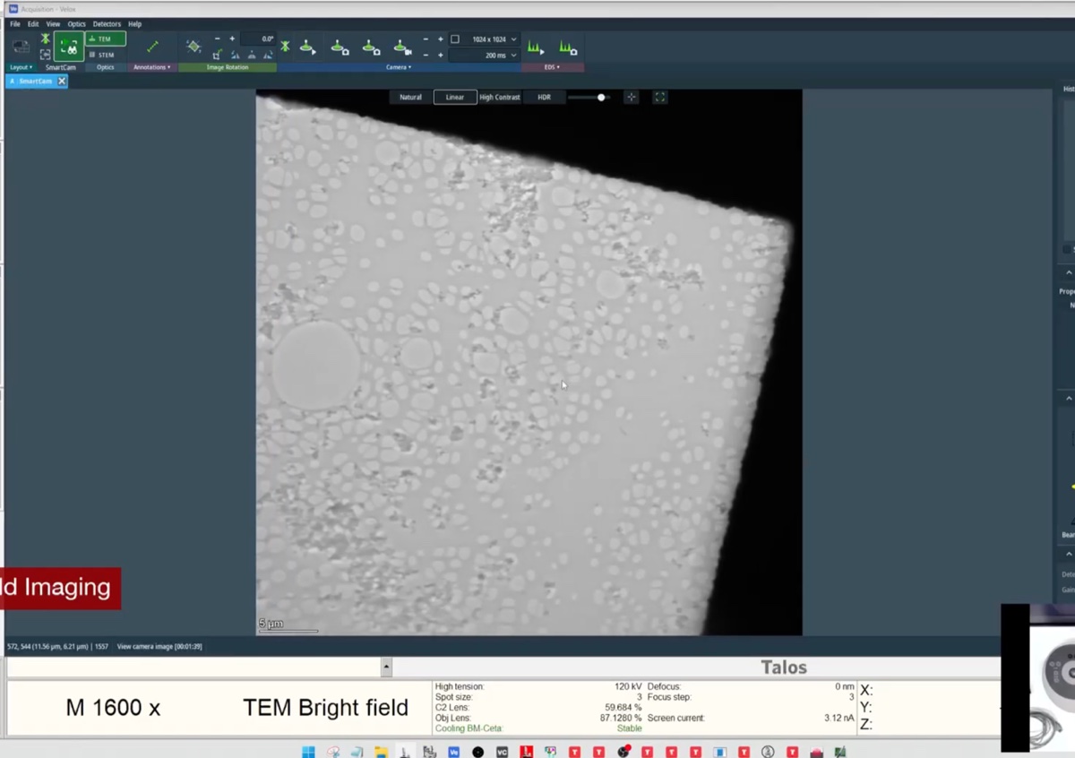
-
Part 5: Dark-field imaging
5.1 Switch the multi-function knob to beam tilt
-
Set mulXY to beam tilt mode
-
Switch the multi-function knob (
mulXY) so that it controls beam tilt rather than stage motion. Beam tilt is the mechanism used to align a chosen diffraction spot onto the optical axis for dark-field imaging.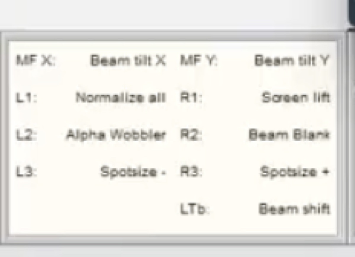
-
5.2 Enter dark-field mode
-
Press the dark-field button
-
Press the dark-field button on the hardware panel to enter dark-field mode.
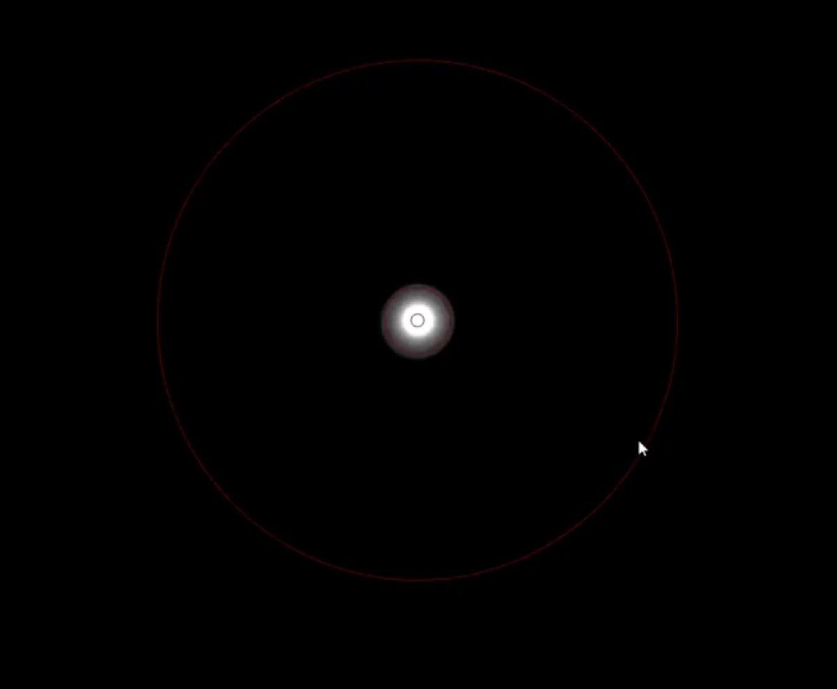
-
5.3 Tilt the beam to align a diffraction spot
-
Align the chosen Bragg reflection onto the optical axis
-
Tilt the beam with the multi-function knob until the chosen diffraction spot sits on the optical axis. In diffraction mode, the central beam and the selected Bragg reflection swap positions when dark-field mode is toggled on.
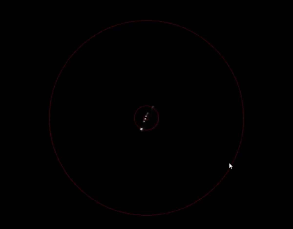
-
5.4 Compare bright-field and dark-field images
-
Acquire matched BF and DF images of the same area
-
Acquire a bright-field reference image first.
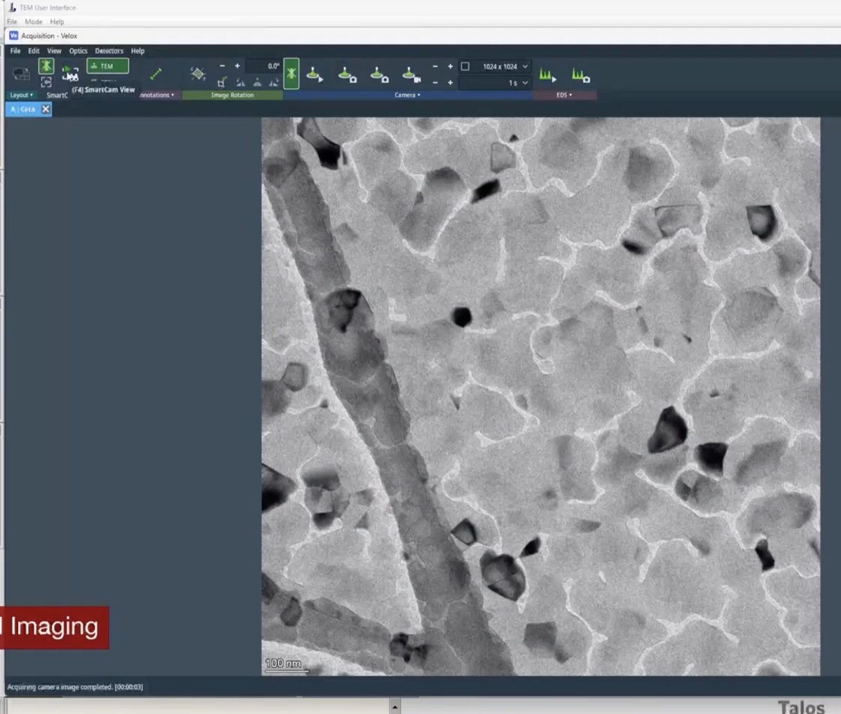
-
Switch back into dark-field mode, leave diffraction mode, and retract the selected-area aperture.
-
Acquire the dark-field image.
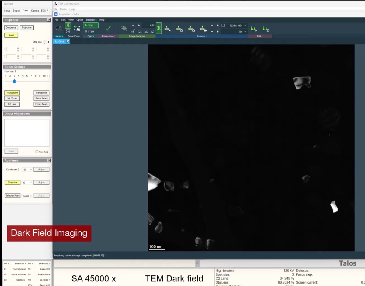
NOTE: Contrast is inverted between BF and DF: grains that diffracted strongly into the selected reflection now appear bright against a dark background.
-
Changelog
- May 11, 2026 : Moved the underfocus/overfocus reference into Session notes since it is session-specific rather than part of the general BF/DF procedure.
- May 11, 2026 : Initial draft compiled from the April 2026 Talos sessions by @bobleesj. BF and DF procedure structure adapted from the existing Phenom Pharos SOP layout.
Drop casting TEM grid preparation
Caution
VERY ROUGH DRAFT, NOT AUTHORITATIVE. This is a personal journey written by @bobleesj (Sangjoon Bob Lee) during his first time drop casting. Photos and notes are his own; the actual experiments were done by Guoliang Hu and Caitlyn Obrero. Terminology, step ordering, and parameter values may be wrong or incomplete. The resulting grids have not yet been imaged to confirm the preparation worked. Treat this page as a starting point to refer back to, not as an SOP. A trained user must verify everything before relying on it.
This page documents how a TEM grid was prepared by drop casting a nanoparticle solution. The grid is first plasma cleaned to make the carbon film hydrophilic, then a small volume of solution is pipetted onto the grid and allowed to dry in air.
Acronyms:
easiGlow:PELCO easiGlowglow discharge / plasma cleanerTEM: transmission electron microscope
Materials:
- TEM grids (e.g., carbon-coated copper, lacey carbon, holey carbon)
- Nanoparticle solution(s) in labeled vials
- Micropipette (0.5 to 10 µL range) with matching tips
- Anti-capillary tweezers
- Glass petri dish lined with lens paper or weighing paper
- Aluminum grid-holder plate for the
easiGlow - Filter paper or lens paper to wick excess solvent
Location
Drop casting is done in the PELCO easiGlow bay in Nucleus Labs W024 (Cryogenic Electron Microscopy) inside the Stanford ChEM-H Building.
The easiGlow workstation sits next to the rotary pump and shares the bench with pipettes, tip boxes, and a gold-sample coupon. Solutions, tweezers, and grid boxes stay on the same bench.
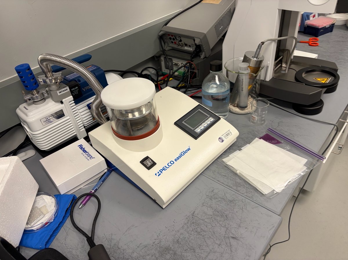
Overview
| Phase | Procedure |
|---|---|
| Part 1: Plasma clean the grids | Load grids on holder, run glow discharge |
| Part 2: Drop cast the solution | Pipette sample onto grid, wick, dry |
| Part 3: Store prepared grids | Transfer dried grids to storage box |
TODO: Record approximate time for each phase once the workflow has been repeated a few times.
Part 1: Plasma clean the grids
Plasma cleaning removes organic contamination and makes the carbon support film hydrophilic, so the aqueous droplet spreads evenly instead of beading up. Skip this step and the solution will roll off the grid or concentrate at the edges.
1.1 Retrieve clean grids
-
Open the grid box
A user must keep grids in a labeled grid box between uses to avoid contamination. Open the box gently: the grids are thin enough that a gust of air can flip them.
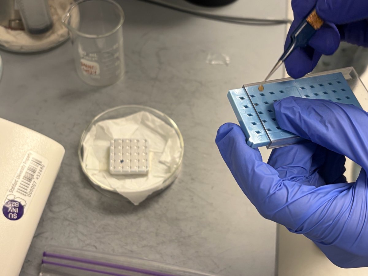
-
Lift a grid with a fine-tip tool
Use a wooden toothpick tip, carbon-tipped vacuum pen, or anti-capillary tweezers to remove a grid. Hold the grid by the edge: pressing on the center will punch a hole through the carbon film.
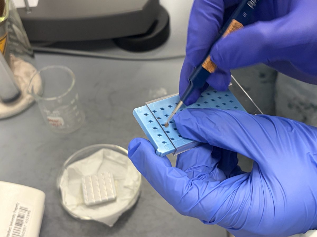
1.2 Load grids onto the easiGlow plate
-
Place grids shiny (carbon) side up on the aluminum plate
The plate has rows of shallow circular wells sized for standard 3 mm grids. Shiny side up ensures the carbon film faces the plasma and becomes the hydrophilic surface.
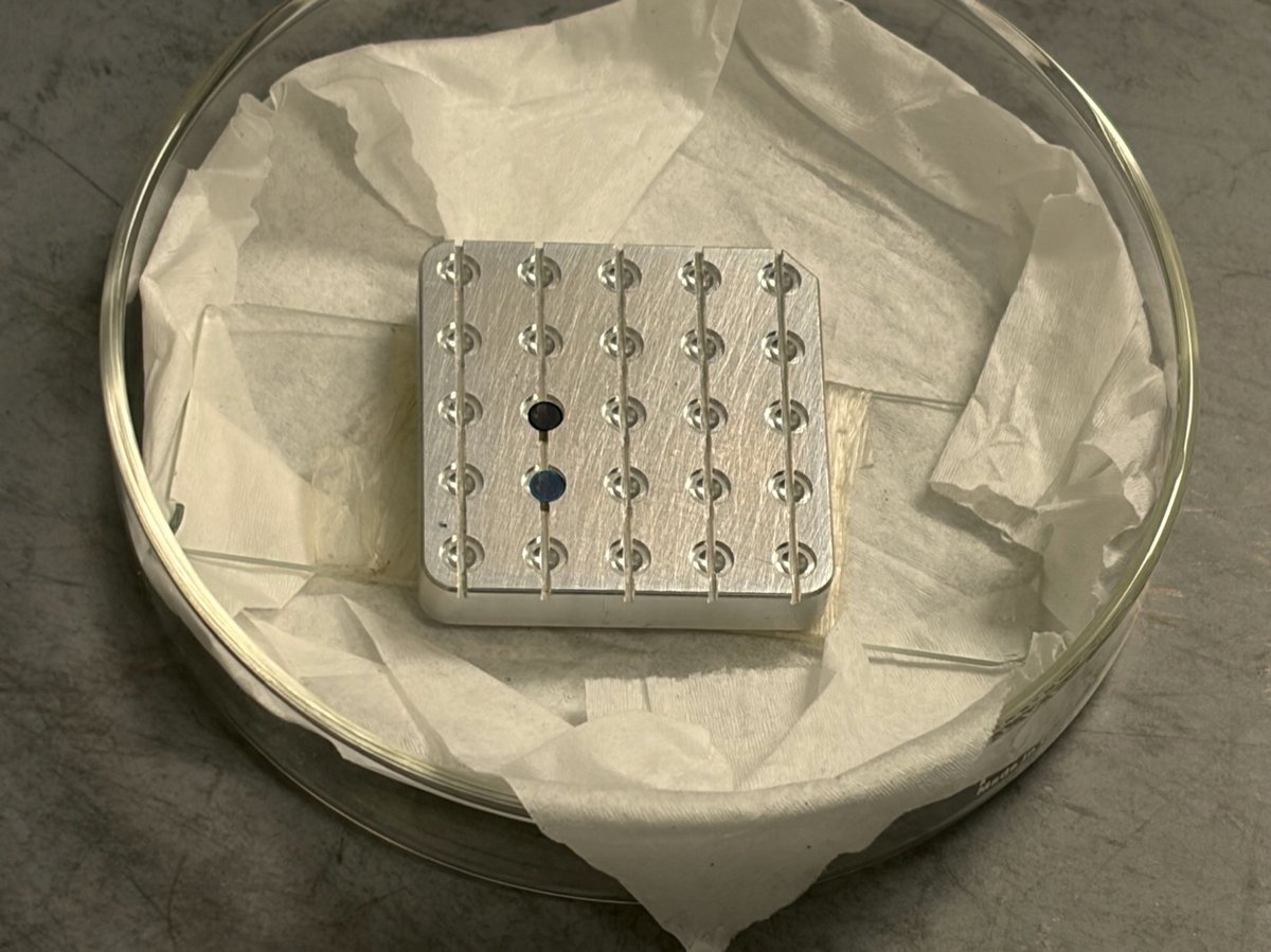
If you cannot tell which side is shiny, tilt the grid under the bench light. The side with the carbon film reflects more uniformly.
-
Transfer the plate onto the easiGlow stage
Slide the plate onto the stainless steel stage inside the
easiGlowchamber. Center it under the upper electrode.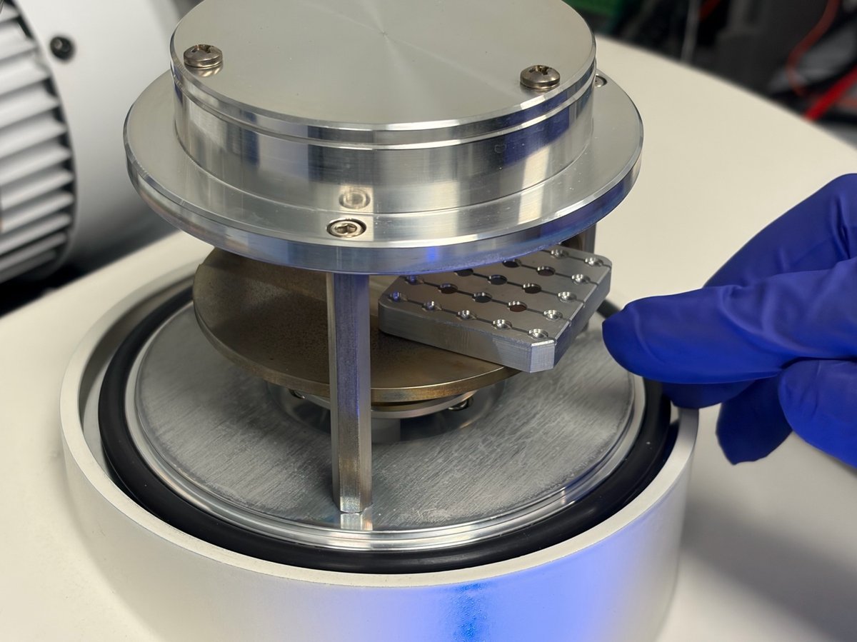
1.3 Run the glow discharge
-
Close the chamber
Lower the bell jar onto the O-ring. Press down gently and evenly until you feel the seal engage.
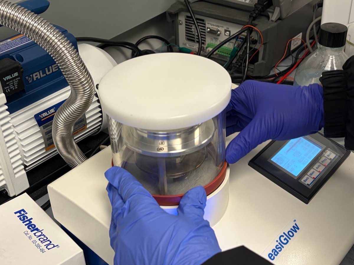
-
Select the negative-glow program on the touchscreen
On the
easiGlowcontrol panel, set the following parameters:Parameter Value Mode NEGATIVEGas GAS 1Pressure TODO: confirm target pressure Current TODO: confirm current (mA) Glow time 60 s Hold time TODO: confirm hold time 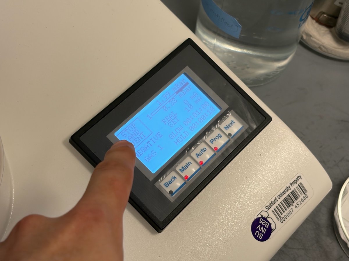
TODO: Record the exact pressure, current, and hold-time values from the staff-defined recipe the next time the instrument is used.
-
Start the cycle
Press
Auto. The pump pulls the chamber down to the set pressure, then the plasma ignites (a faint purple glow appears inside the bell jar). The cycle auto-vents at the end. -
Use the grids promptly
Plasma-cleaned grids lose hydrophilicity over time as the surface re-adsorbs ambient hydrocarbons. Prepare your solution and pipette tips before starting the glow discharge so you can drop cast immediately.
TODO: Confirm how long after glow discharge the grids remain usable.
Part 2: Drop cast the solution
2.1 Prepare the solution
-
Check that your sample vials are labeled and in a rack
Each vial should have a unique label (e.g.,
S1-3,S2-1) matching your lab notebook. Vortex or gently invert any solution that has sat for more than a few minutes to resuspend settled particles.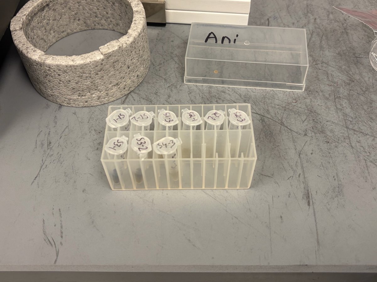
-
Mount a fresh tip on the micropipette
Use a tip that matches your pipette (e.g.,
SL-10 XLS, 0.5 to 10 µL). A fresh tip prevents cross-contamination between samples.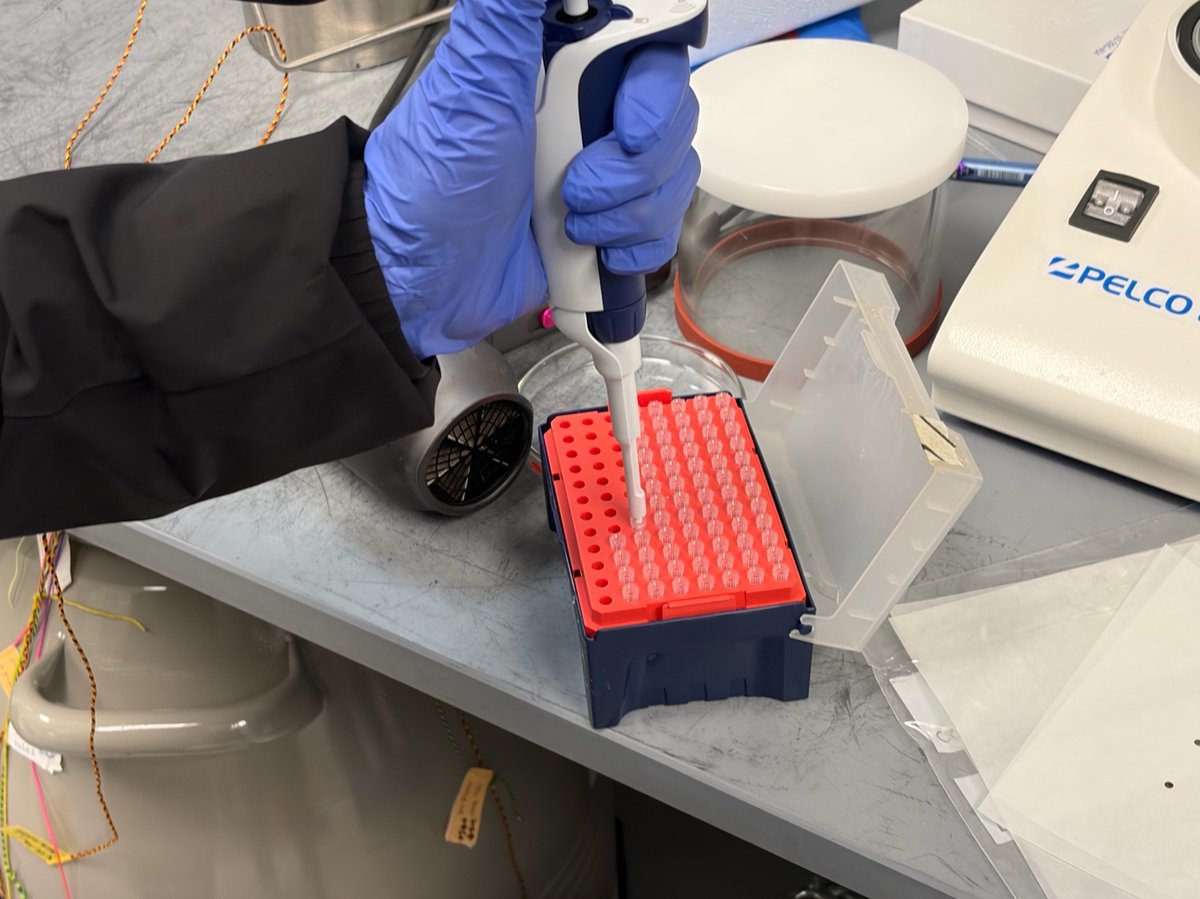
2.2 Pipette onto the grid
-
Draw solution from the vial
Press the plunger to the first stop, dip the tip into the solution, and release slowly to draw the volume. Avoid drawing air: a bubble at the tip will spray the droplet off the grid.
TODO: Record the volume actually used (microliters) and the pipette model/range.
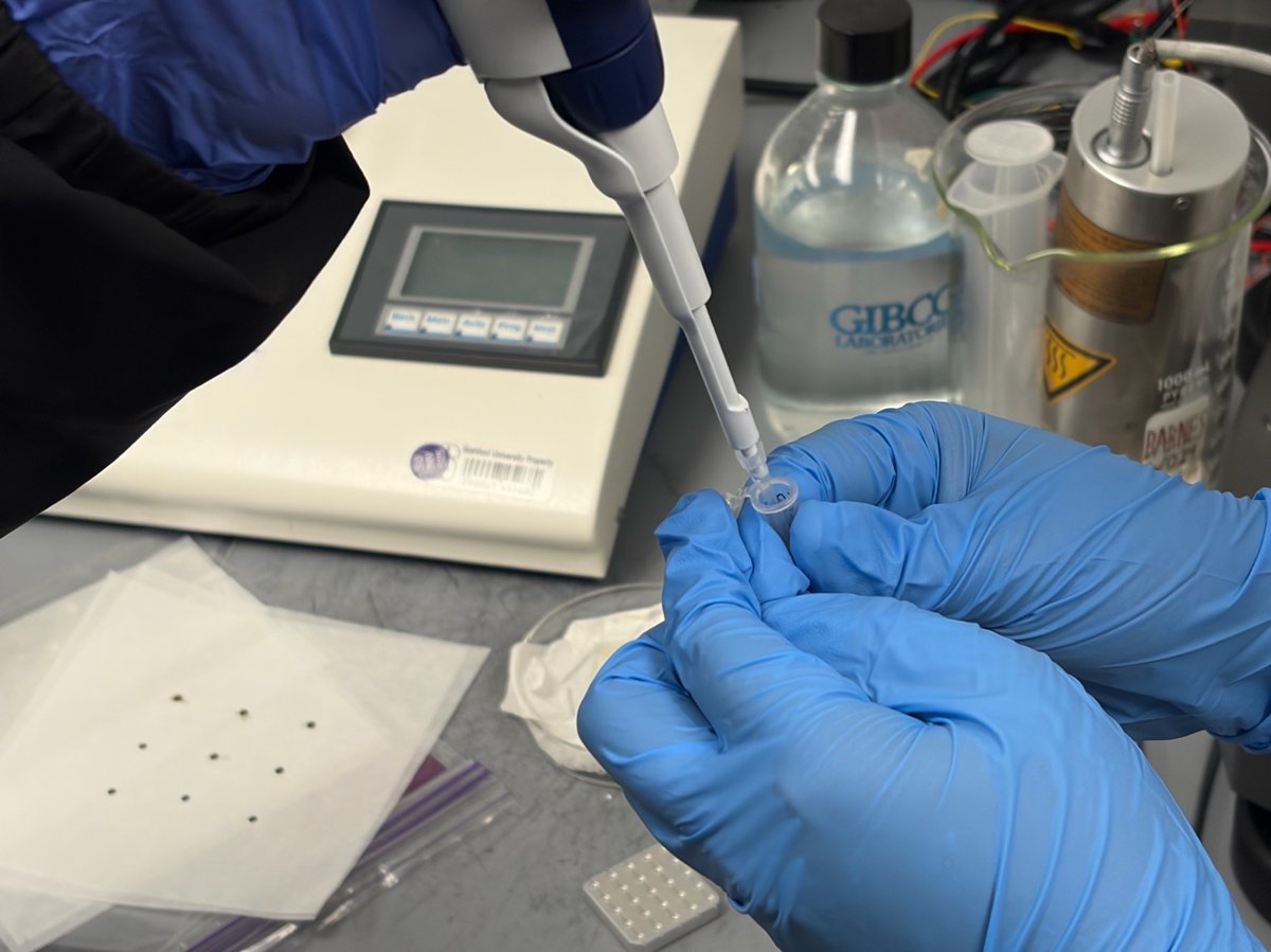
-
Deposit the droplet on the grid
Hold the pipette vertically above the grid. Touch the droplet to the grid surface so it wets across the film. Do not press the tip into the carbon film.
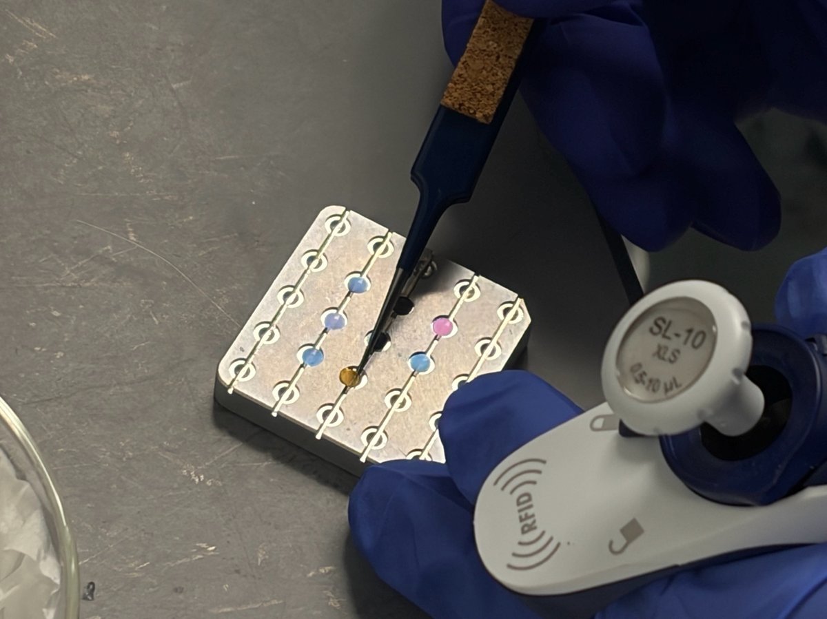
If the droplet beads up and rolls off, the grid was not plasma cleaned recently enough. Repeat Part 1 with a fresh grid.
2.3 Wick and dry
-
Transfer the grid onto a piece of lens paper
Place the grid sample-side up on clean lens paper or filter paper. The paper wicks excess solvent from the edges without disturbing the deposited particles.
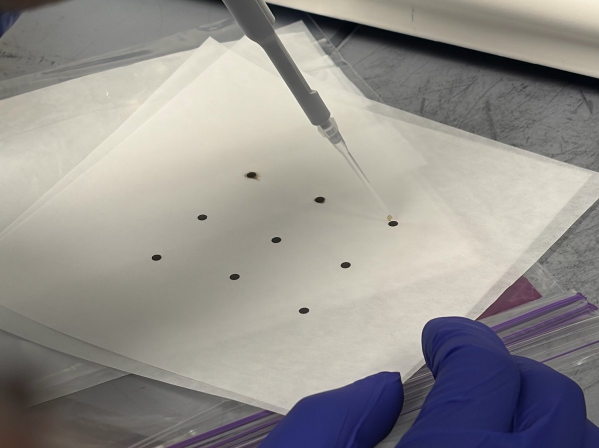
-
Let the grid air dry
Wait until the droplet is fully evaporated. Drying time depends on the solvent and droplet volume.
Do not blow on the grid to speed drying. Breath moisture deposits contamination, and forced airflow can redistribute particles asymmetrically.
TODO: Record actual drying time for the solvent(s) used.
Part 3: Store prepared grids
-
Pick up the dried grid with anti-capillary tweezers
Grip the grid by the edge only. The dark dot visible in the center is the dried sample: touching it will scrape particles off.

-
Return the grid to a labeled grid box
Note the well number and sample ID in your lab notebook.
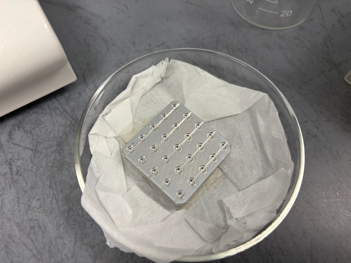
Troubleshooting
TODO: This table is generic drop casting guidance, not validated against the actual SNSF workflow. Verify with Guoliang Hu or Caitlyn Obrero before relying on it.
| Symptom | Likely cause | Action |
|---|---|---|
| Droplet beads up and rolls off | Grid not plasma cleaned or surface re-contaminated | Re-run glow discharge with a fresh grid |
| Particles concentrated at droplet edge (coffee-ring) | Solvent evaporated too slowly or grid not level | Reduce droplet volume, or wick the edge with filter paper |
| Carbon film torn | Pipette tip touched the grid | Lower the droplet without contacting the film |
| No plasma ignition | Chamber not at base pressure | Reseat the bell jar, wipe the O-ring |
| Visible aggregates on grid | Solution not resuspended | Vortex sample, dilute, repeat |
Changelog
- Apr 22, 2026 - Initial draft captured during first drop casting session. Photos and notes by @bobleesj. Experiments by Guoliang Hu and Caitlyn Obrero. Output not yet verified by TEM imaging.
Sample loading
Location
TITAN:
Sample loading is done outside of the room where Titan is hosted:
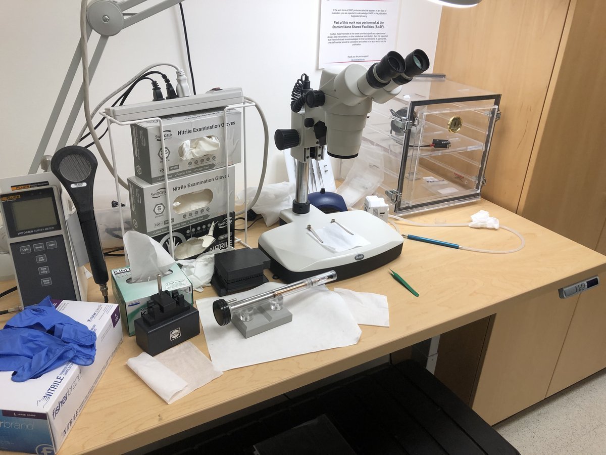
Spectra 300:
Sample loading can be done inside the Spectra room:
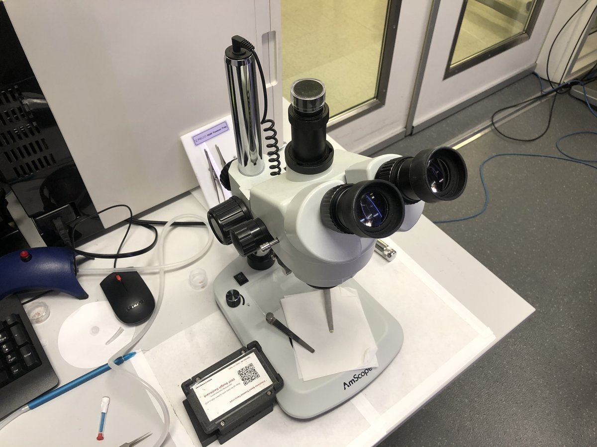
Sample holders are stored here at room temperature:

Single-tilt holder
Load sample:
FIXME: use technical terms for these objects… “pin” or “clip”?
-
Push the pin inside the tiny hole shown below:
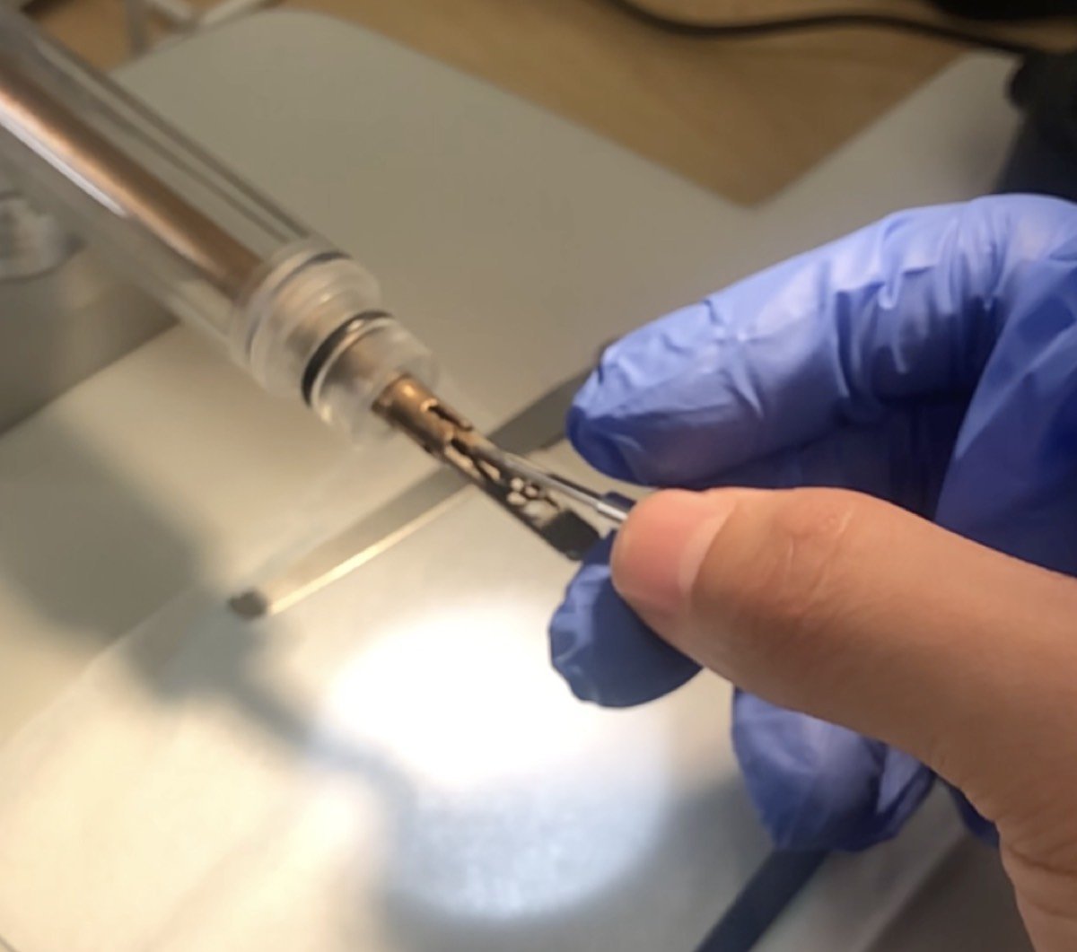
-
Lift the clip gently:
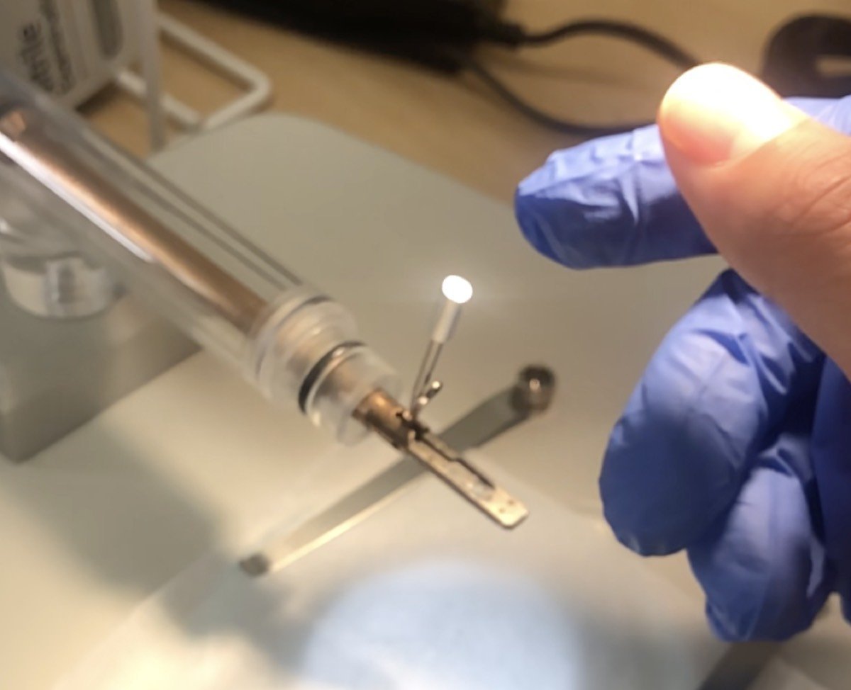
-
If using a copper grid, pinch the tip of the copper grid
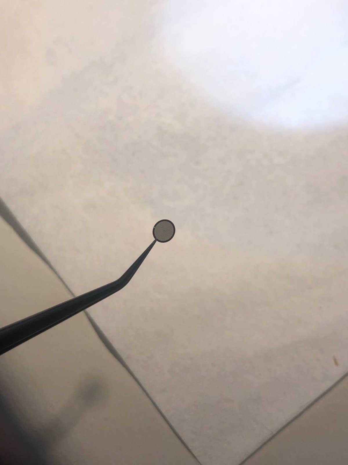
-
Place the sample, shiny side up for the standard sample
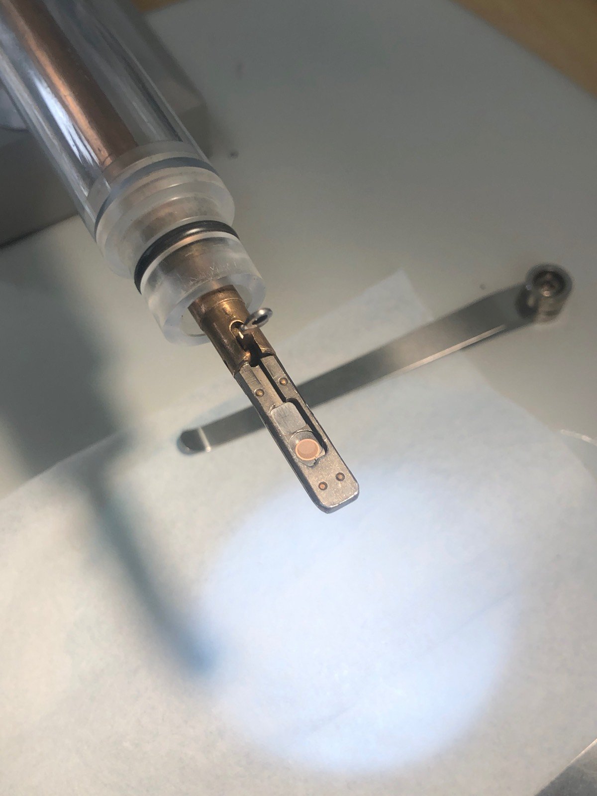
Double-tilt holder
Load sample:
-
Load the sample and washer (gold donut):
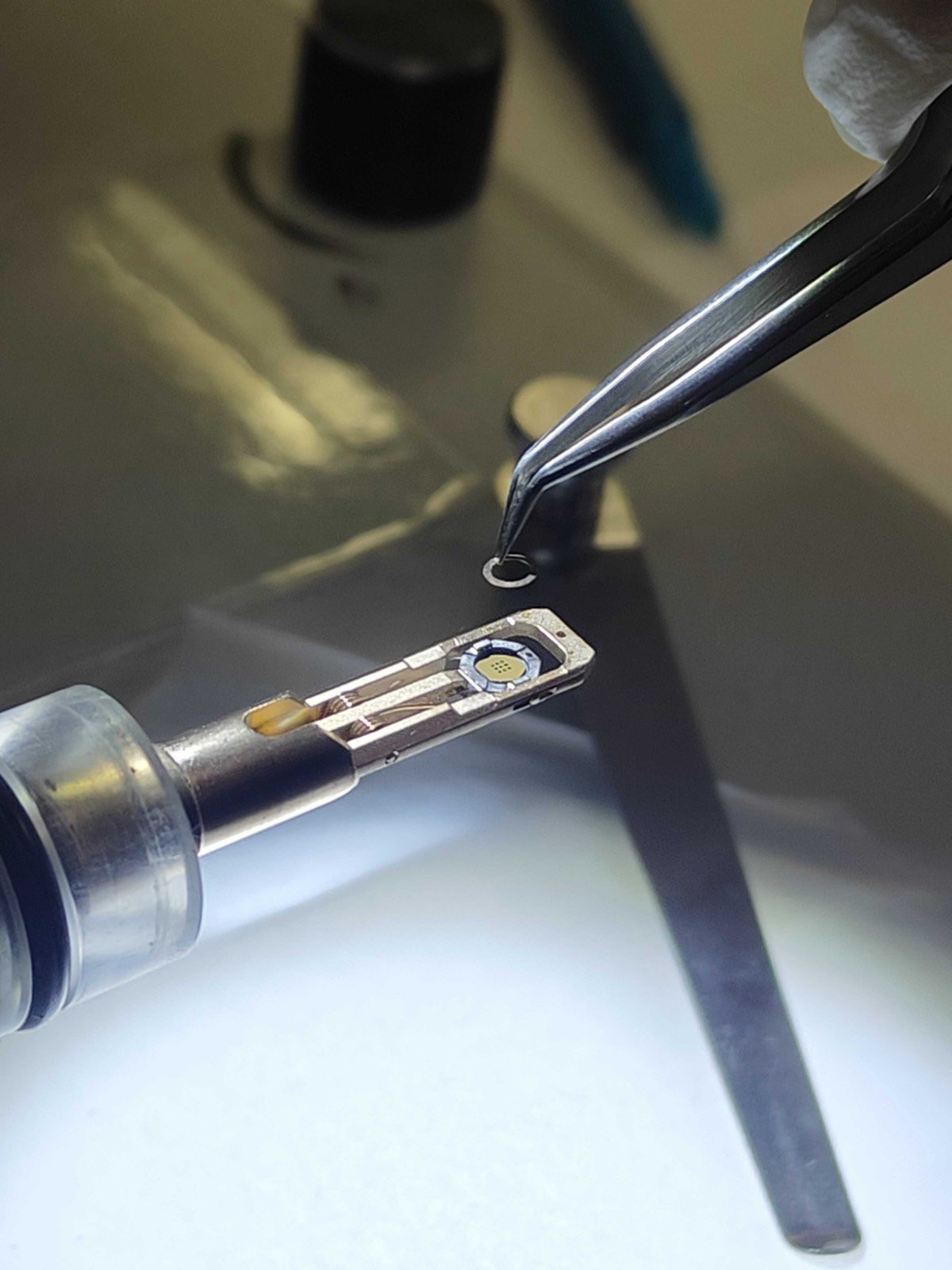
-
Add the cap and rotate the holder about the long axis to ensure the sample is secure:
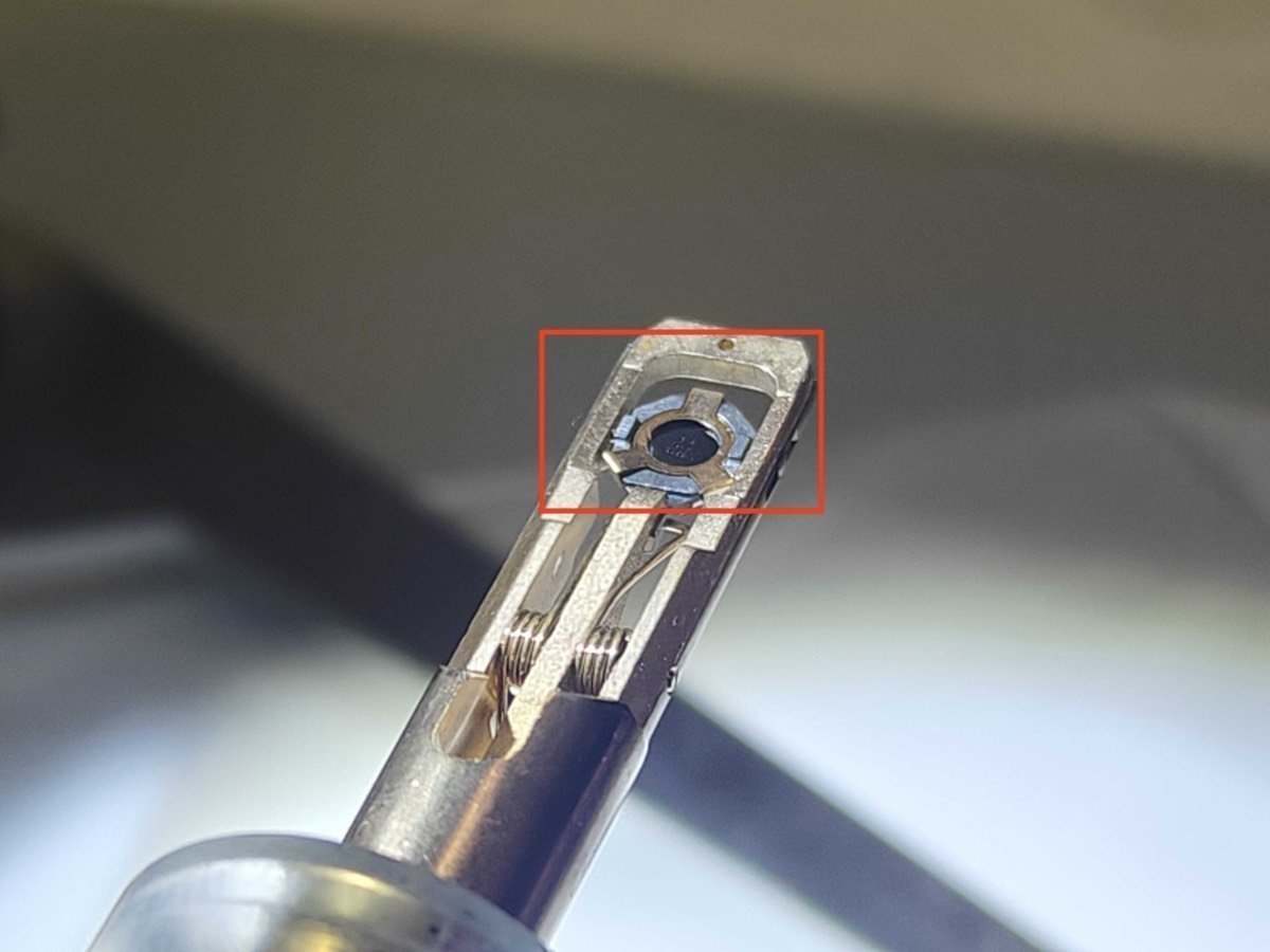
Unload sample:
-
Press down the very small hole gently as shown below:
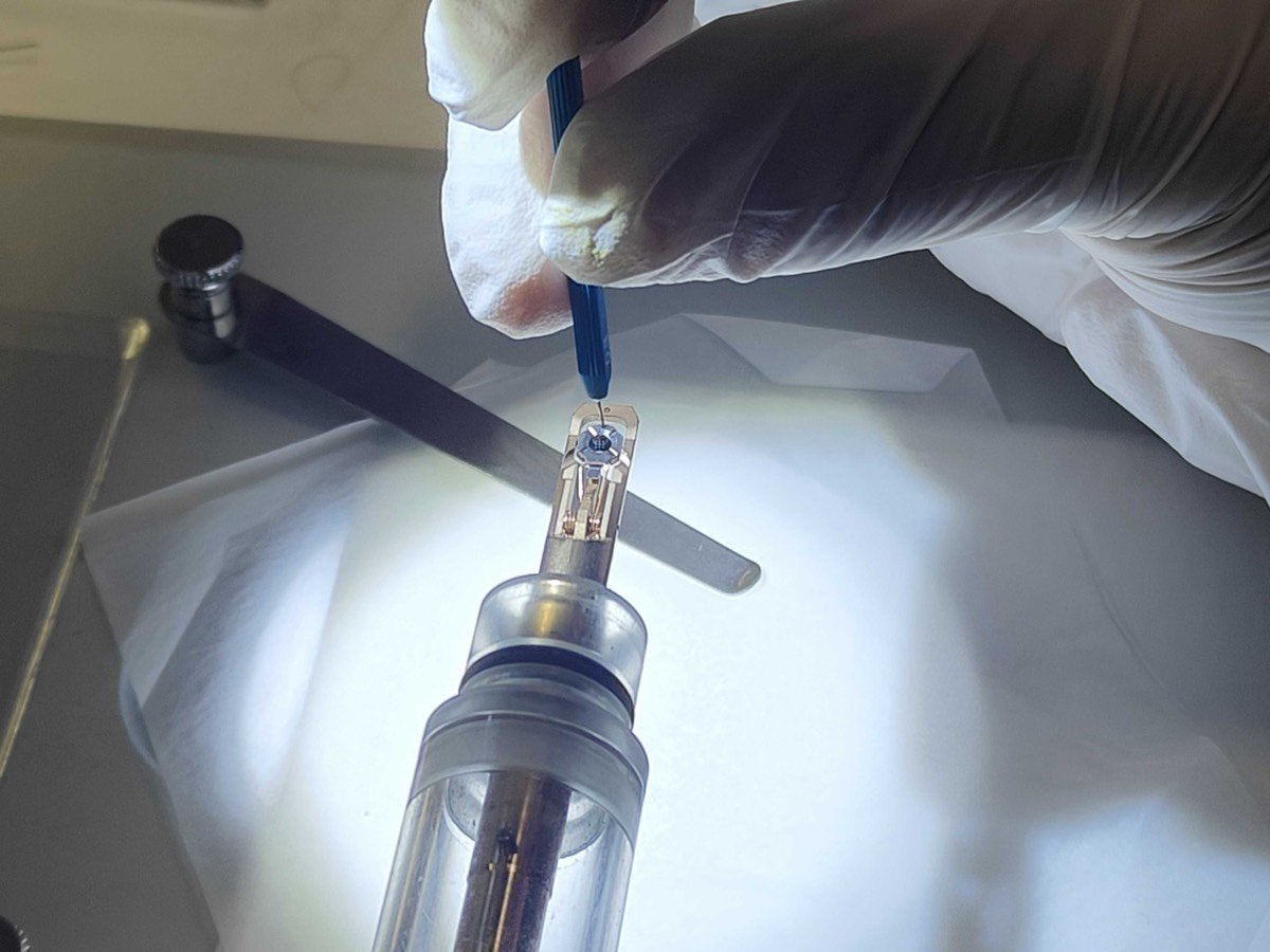
-
The three parts should all be disassembled and placed on the bottom:
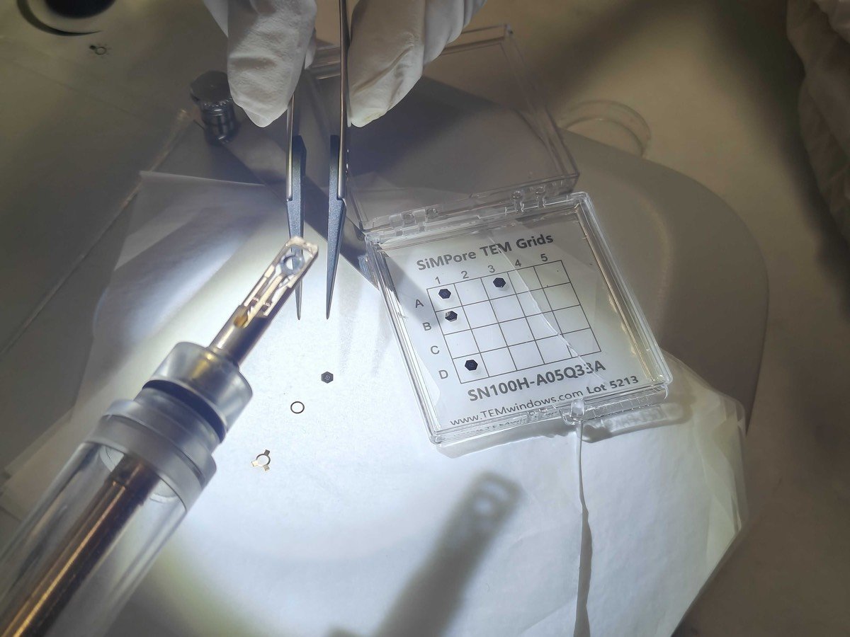
Tomography holder
Unload sample
-
The sample grid is held between the two “arms” of the metal strips.
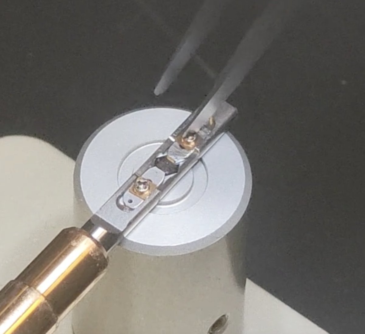
-
Rotate the screw counterclockwise about 90 degrees. Repeat for the other “arm”.
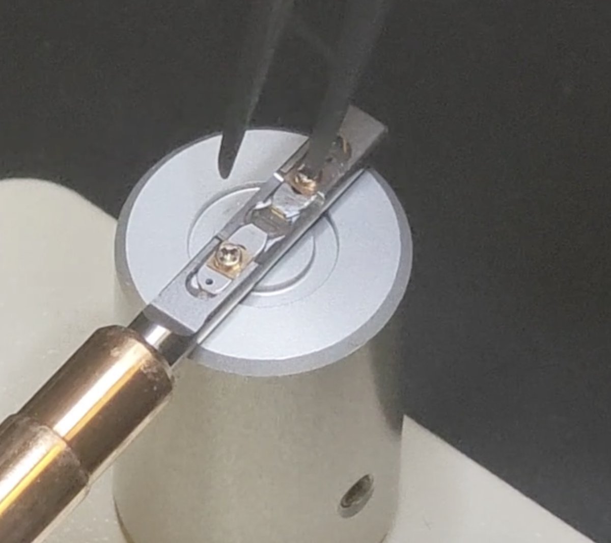
-
Move the two strips away from each other to free the sample
From:
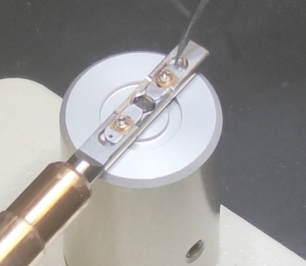
To:
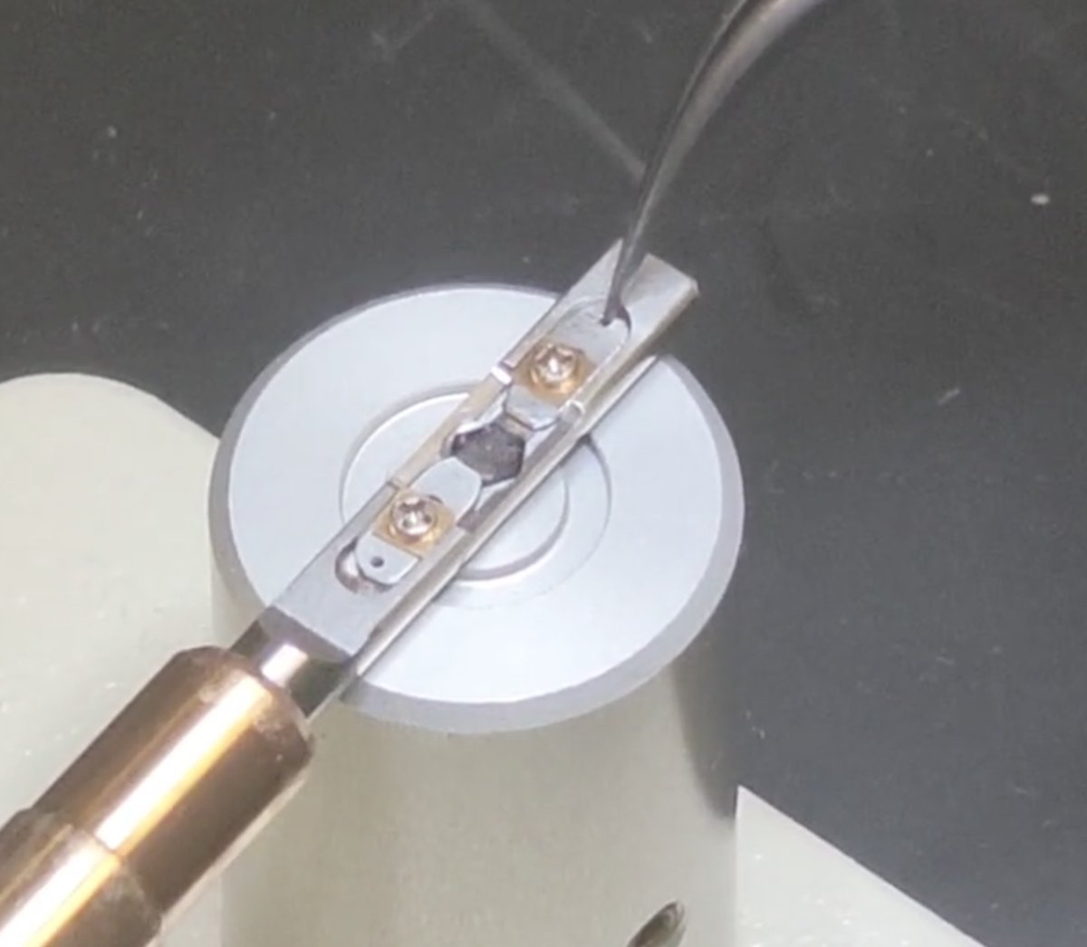
-
Remove the sample
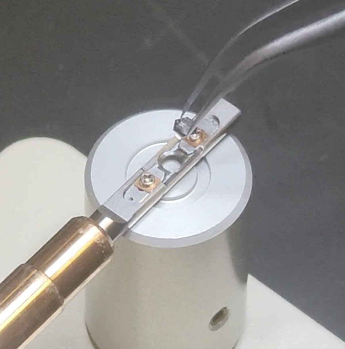
Load sample
Follow the process in reverse: load a new sample, pull the two strips closer together, and rotate the screws clockwise.
Changelog
- Dec 20, 2025 - Rnhance holder insersion process with visuals
- Dec 18, 2025 - Reorganize into Start/End session sections for use across all tutorials by @bobleesj
- Dec 17, 2025 - Add sample loading region by @bobleesj
- Dec 15, 2025 - Add tomography holder section by @bobleesj, with images taken by Guoliang Hu
- Dec 13, 2025 - Add single-tilt, double-tilt holder section by @bobleesj, with images taken by Guoliang Hu
Share Your Procedure
We want to bring electron microscopy techniques and SOPs together across institutions.
Why contribute?
- Seamless experiments - Researchers traveling between facilities can quickly get up to speed on different microscopes
- Reduced friction - Standardized visual guides reduce training time and errors
- Community knowledge - Your expertise helps the broader EM community
What we’re looking for
- Step-by-step operating procedures for your microscope
- Visual guides with screenshots or photos
- Tips and tricks from experienced operators
- Troubleshooting guides
How to contribute
We can help with writing, formatting, and organizing your content. You don’t need to be a programmer!
- Prepare your notes - Word docs, Google Docs, handwritten notes, photos from your phone - anything works
- Reach out - Contact @bobleesj or open an issue on the GitHub repo
- We’ll handle the rest - We’ll format your content and add it to the site under your institution’s section
Institutions we’d love to hear from
- National labs
- University facilities
- Industry labs
- International facilities
Your procedures will be credited to you and your institution.
Changelog
- Dec 18, 2025 - Page created
Session notes
View from Hoover Tower, Stanford, Mar 24, 2026
by Sangjoon Bob Lee
This is a working scratchpad for raw notes taken during microscopy training visits and sessions. Notes here capture practical tips, questions, and observations from hands-on time at the instrument. Over time, useful content gets refined and incorporated into the proper guide sections.
Open questions to verify at the microscope
- For C1A1, during the first run, what are the target values? I started with C1 6 nm, A1 27 nm, B2 928 nm. My notes say C1 < 1 nm and A1 < 3 nm. Add target values to the table.
- Add a table at the beginning with the target values for aberration corrections.
- When to change condenser stig? Need to verify on the Spectra what the beam looks like before and after condenser stigmator correction.
- What is the minimum correction quality needed for atomic resolution?
- Investigate the effect of descan when you integrate or sum across k-space.
Hands-on practice (need to do on my own)
- Try going back to TEM and STEM, confirm aberrations getting worse.
- Try going to LM and then back to regular STEM, confirm resolution getting worse.
- Try correcting the probe without Sherpa, in the case of beam sensitivity.
Answered
- (Apr 3) When do you run Stigmator? Both with the ronchigram (diffraction mode) and directly in HAADF imaging (probe image mode).
- (Apr 3) When do you do manual tuning? Yes, with real samples when Sherpa can’t be used. See Aberration Correction (Advanced).
- (Apr 3) Figure out the full workflow for correcting aberrations without Sherpa. See Aberration Correction (Advanced).
- (Apr 3) Where do you run C1A1 if you can’t expose the sample? Run on the gold standard first, then switch to your sample. See Aberration Correction (Advanced).
- (Apr 3) What does “good” look like without Sherpa? See What a good probe looks like in the Mar 25 session.
Apr 23, 2026: Underfocus vs overfocus on the Talos (MATSCI 322)
A short follow-up session in the Stanford MATSCI 322 TEM Lab (with Andrew Barnum, Pinaki Mukherjee, and Ash) to nail down what under- and over-focused images actually look like on the Talos FluCam, using latex spheres as the test object.
Underfocus
Turn the intensity knob counter-clockwise from focused crossover. This strengthens the C2 lens (C2 current increases), which is underfocus from the C2 lens perspective: the C2 focal point moves upward relative to the eucentric height (negative defocus relative to eucentric).
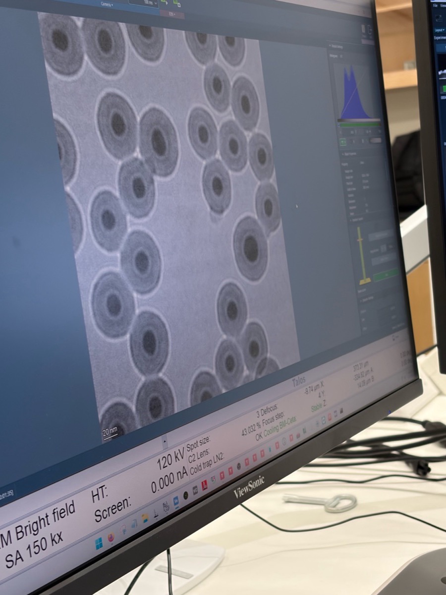
Visual signature: a bright ring on the outside of each sphere.
Overfocus
Turn the intensity knob clockwise from focused crossover. This weakens the C2 lens (C2 current decreases), which is overfocus from the C2 lens perspective (positive defocus relative to eucentric).
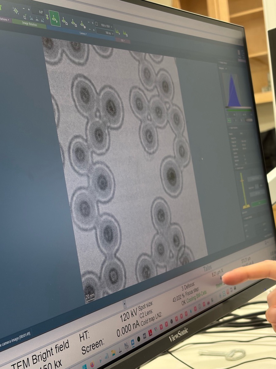
Visual signature: a bright ring on the inside of each sphere.
The two sign conventions are opposite
- From the C2 lens perspective, “underfocus” means the lens is stronger (C2 current up); “overfocus” means weaker (C2 current down).
- From the beam perspective, “over” means the focal plane is past the sample, so the “over” region sits below the sample.
Record which convention is in use when interpreting a defocus value during a session. Treat the eucentric height as the source of truth: a calibrated defocus reading on the instrument is given relative to the eucentric position.
Apr 3, 2026: Time-series for beam sensitive and low contrast at SNSF
I implemented live SSB reconstruction and also learned to fill up nitrogen in Spectra. Today, I joined Parivash Moradifar’s session to shadow for manual aberration correction, and Dasol’s session for beam-sensitive sample imaging.
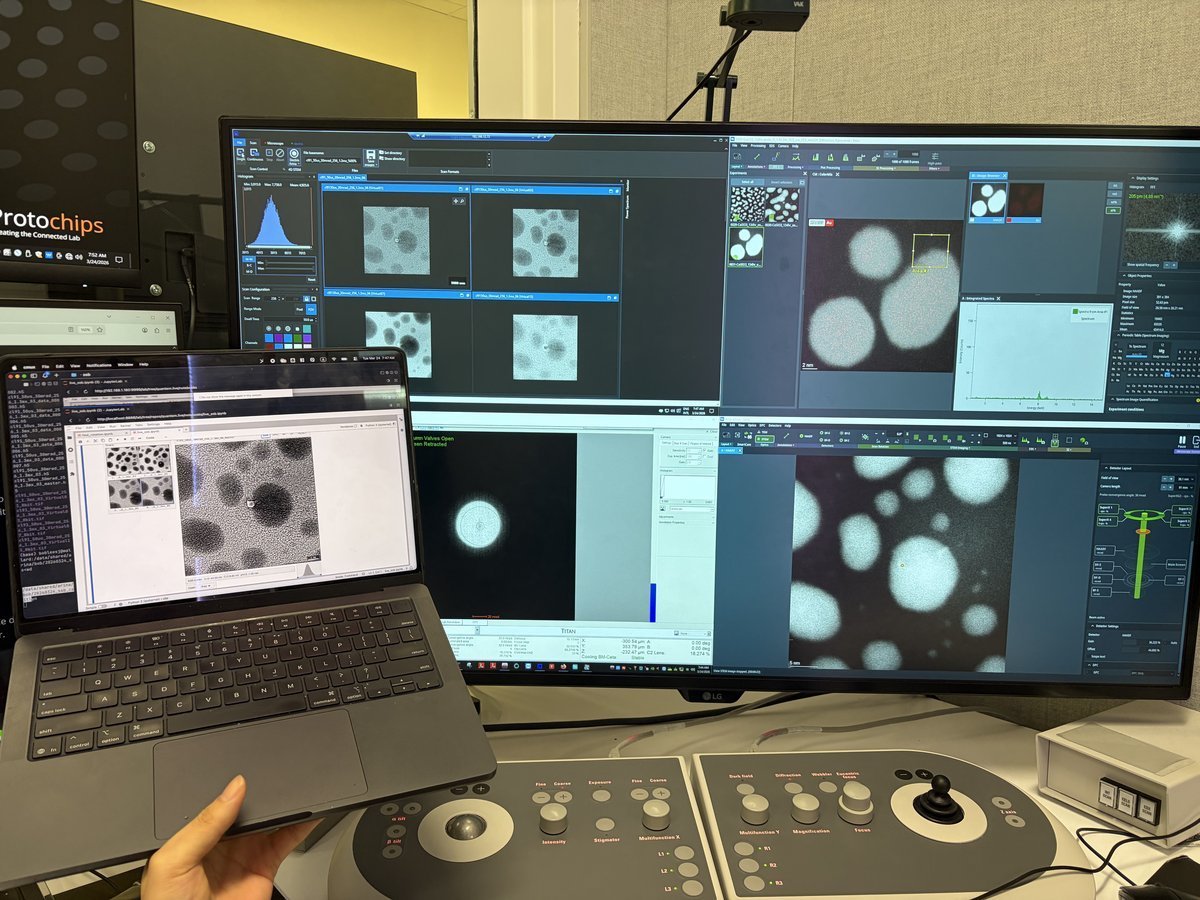
The benefit of live SSB is that you can also find the gold zone axis and verify crystallographic orientation from the reconstruction, not just from the ronchigram.
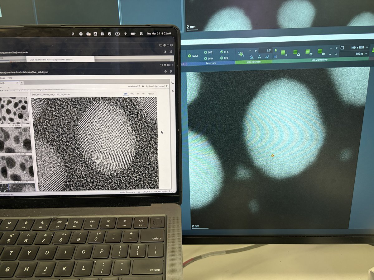
- We encountered a thick silicon nitride grid (~100 nm) that interacts with the incoming electrons. Silicon nitride grids are sinuous, so the resulting images look jiggly.
- I also learned how to reduce contamination via beam shower. It is typically done in TEM. In STEM mode, go to really low defocus using z-axis and have current around 0.200 nA. It will reduce contamination.
Mar 25, 2026: Spectra 300 imaging quality after probe correction at SNSF
Spectra 300 at SNSF after completing the full STEM alignment and aberration correction on the gold nanoparticle standard sample. The HAADF image provides a standard.
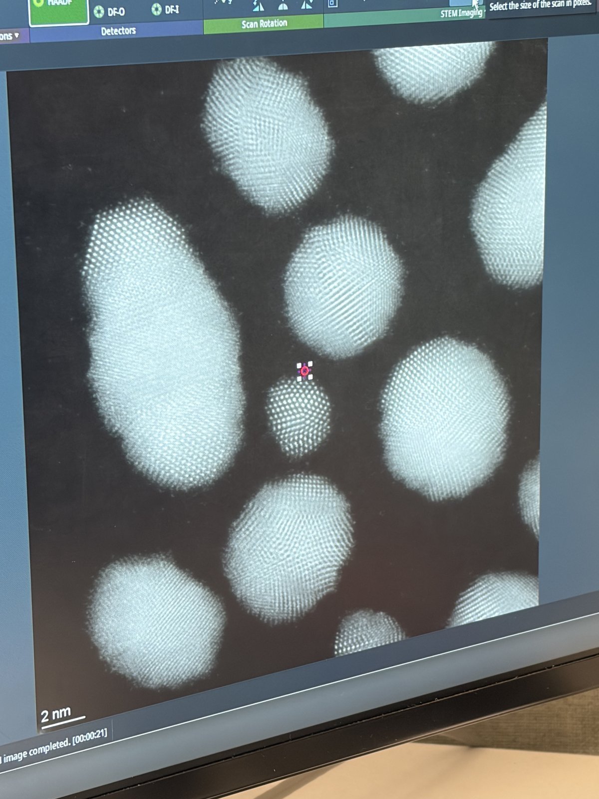
The FFT confirms 74.5 pm resolution (4096x4096 image, pixel size 6.579 pm, 26.95 nm field of view).
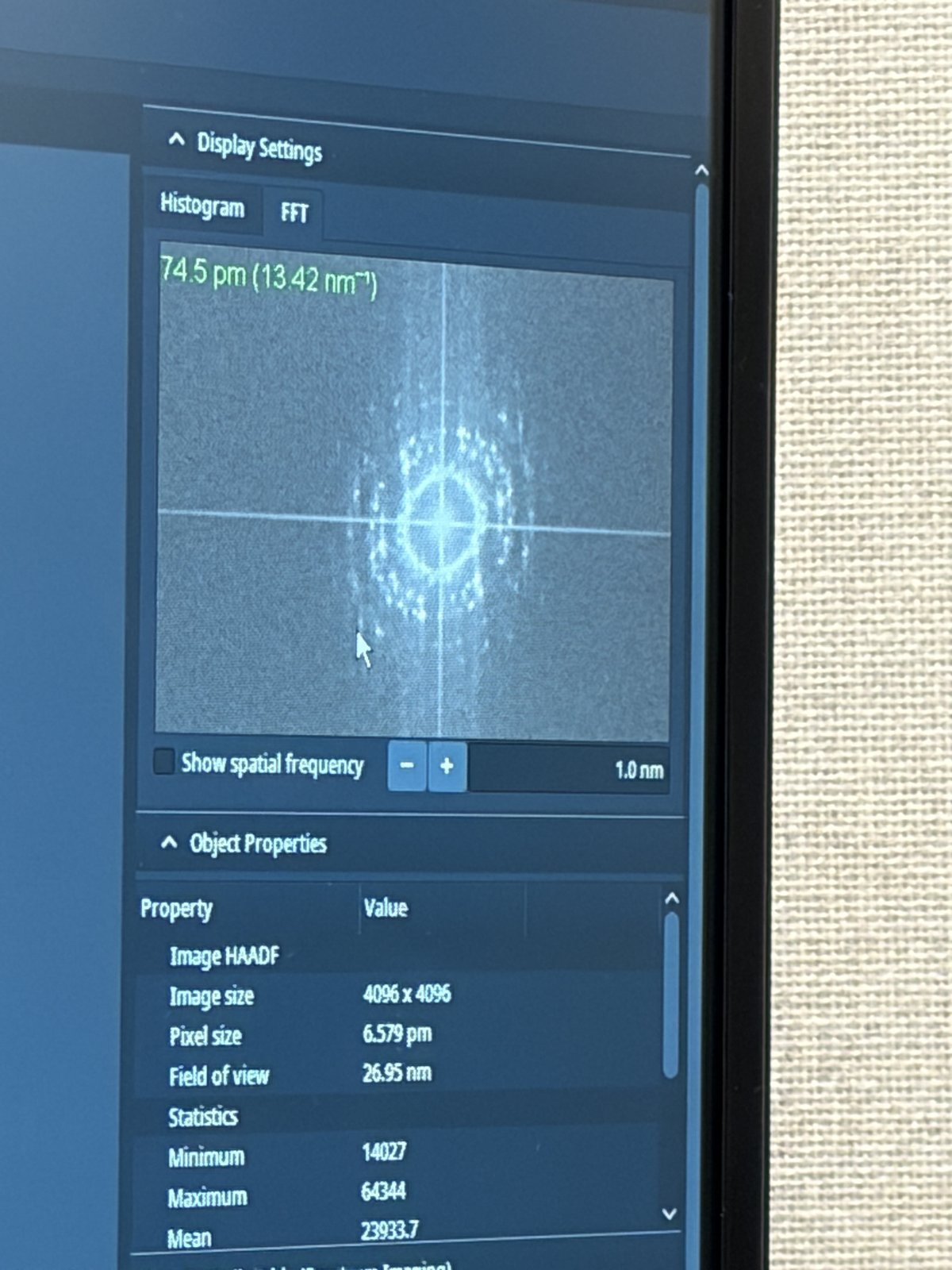
What a good probe looks like after aberration correction:
Tableau measurement showing under-focus and over-focus ronchigram tiles. Each tile should show a round, symmetric probe. The C1A1 values at the bottom show the aberration measurements converging.
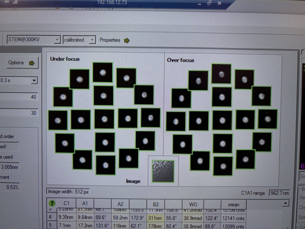
State of correction showing the aberration table and phase plate. The phase plate (green/purple visualization) should show a flat, symmetric pattern within the semi-aperture circle. Probe current is 161 pA, semi-aperture 30 mrad, probe size 40 pm.
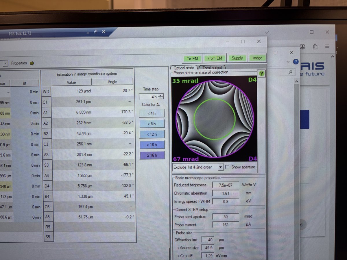
Ronchigram after correction. This is considered good: the featureless central region is large, round, and extends well beyond the 20 mrad scale bar. The red circle marks the semi-aperture boundary.
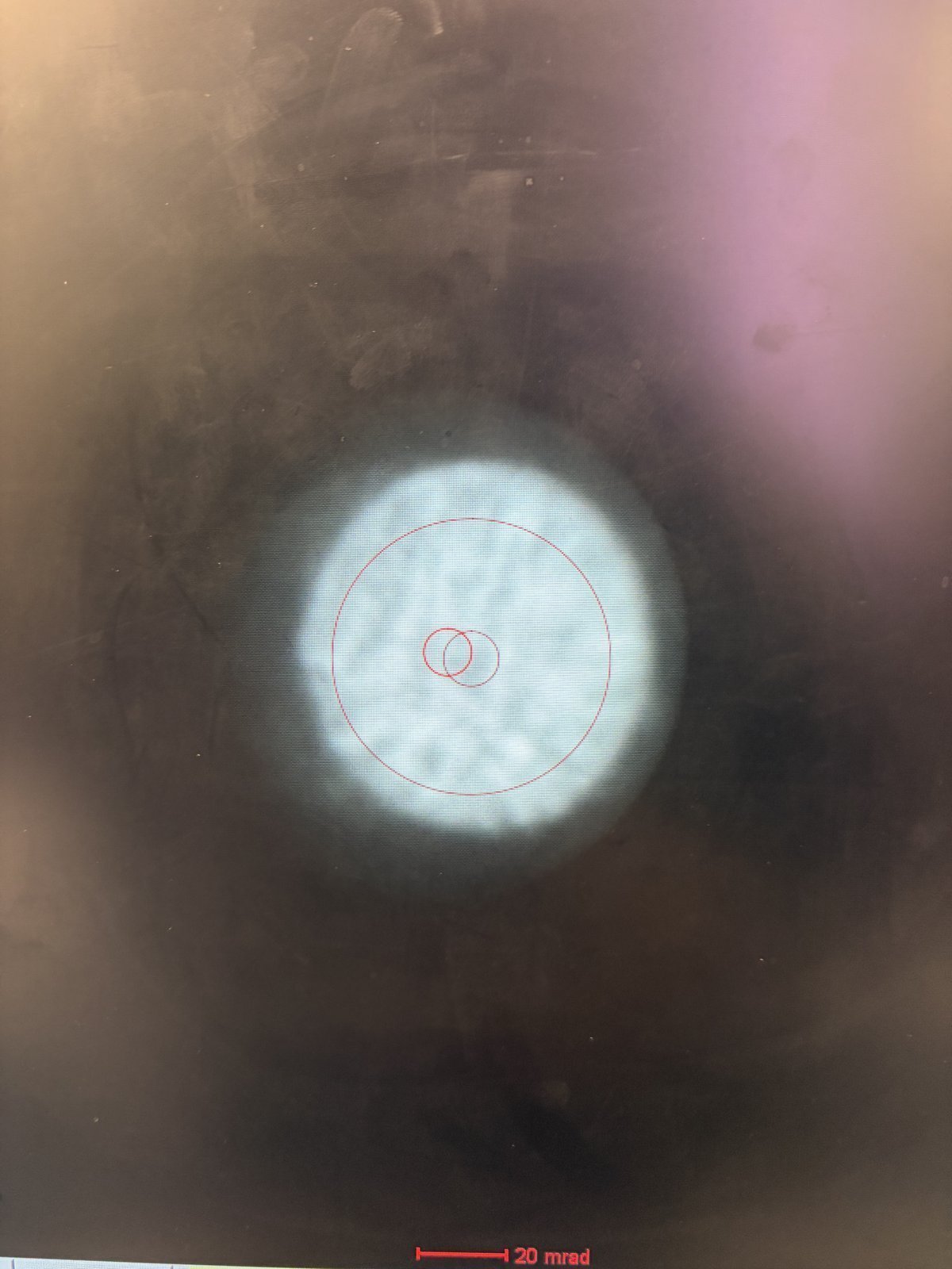
Mar 14, 2026: Improve resolution using the Spectra SOP and feedback
How to find the ronchigram again?
- Move the joystick around and watch for a small screen current change.
- Then use Diffraction Shift and Focus alignment to find the beam. You will see a faint bit of light.
Open questions
- Ideal Velox play setting? 1024x1024 and 500 ns for gold standard sample.
- Camera length and ronchigram size? Proportional: 91 mm to 115 mm, ronchigram size also increases.
- When do you adjust Condenser?
Lessons learned
- Beam condition from FFT: 4-6 rings, each ring with discrete peaks, ~70 pm. Further rings (bigger k) correspond to sharper features resolved in real space.
- Beam condition from Probe corrector: flatness around the “green” aberration surface is the key.
- Overfocus means focal point above the sample; underfocus means below it.
- Defocus change DP? Barely, but real-space probe size is changed (needed for ptycho overlaps).
- Defocus on BF? Expect it to get worse. Ptycho will perform better.
- Focus knob to sharpen? Minimize it. Don’t add degrees of freedom. 20 nm max, use stage piezo and knobs.
- Finding ptycho defocus step size: use ronchigram shadow image to determine feature size variations. Step size of 1 nm is too small.
- Why drift? Inserting the holder itself induces aberrations. After stage movement, find ROI, then wait ~5 min for mechanical stabilization.
Extra notes on aberrations
- Practice getting atomic imaging without Sherpa. Example: Samsung sample, too beam-sensitive for Sherpa.
- Tableau with A5 selected measures up to 5th order aberrations.

Mar 9, 2026: Ptychography reconstruction basics
Notes from Arthur on reconstructing data collected from ARINA detector at Stanford.
- Sign convention: in
quantem,C10 > 0means underfocus. The beam focal point is below the sample, hence negative defocus. - Aberrations: SSB is somewhat an “eye test.” One may use the aberrations from SSB or not. There are many degrees of freedom: batch size, the “dose” step size (finer can be better), probe size, center of mass/transpose, and initial aberrations.
- Cropping strategy: in real space, it’s fine to crop, encouraged since faster. In k space, we generally don’t want to crop since we lose the max scattering angle, i.e. we lose fine details in real space.
- Probe: aberrations should be identical across all scan regions in theory. However, for ptycho-tomo, defocus will change with tilt.
- CNN reconstruction: reconstruction weight is different between reconstructions since these are weights being trained.
- Memory: It’s hard to manage memory well in Jupyter notebook but it’s something we can work on.
- Virus samples: there is no zone axis, so we can’t do atomic resolution.
- Descan: the beam is tilted from the source and then tilted back after a short travel perpendicular to the sample. During this second tilt, instability can be introduced and the diffraction pattern isn’t perfectly aligned.
- Mixed probe: mixed probe is good and orthogonality is imposed, so probes should look different from each other.
Mar 3, 2026: My cobalt oxide nanoparticles 4DSTEM at SNSF
It was my first time staying in STEM mode and find samples after STEM probe correction and loading my own sample. The following notes were taken in my attempt to find the feature of interest right after the sample was loaded.
- Go to 5,000× magnification. If there is no beam, it means the beam is blocked on the grid. Move the stage around with the joystick.
- Move the stage until the screen current increases to about 0.150 nA. At this point, the beam has been found. Notice the Kikuchi bands: this is a good clue that you are in a good starting place.
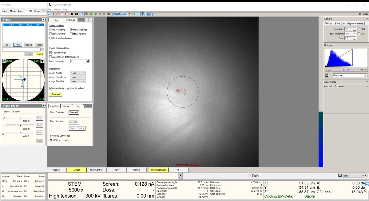
- Increase the magnification to 20,000× or higher. The features will still look blurry since we are not yet at the correct focus.
- Press the Z-axis up and down until the Ronchigram blow-up point appears. Adjust z-axis from 5kx to 20kx to find the blow-up point.
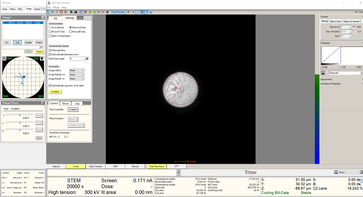
- After the blow-up point, you will see features. In this session, cubes were found after the Ronchigram blow-up point.
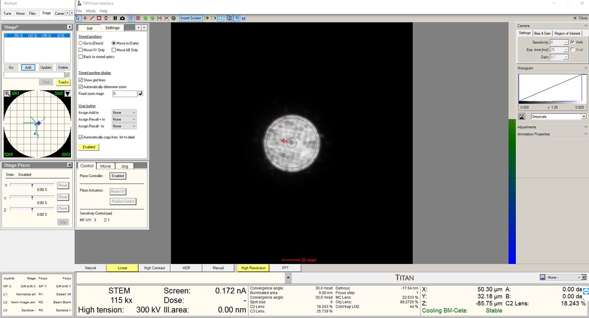
- Stay at the blow-up point. We are now at the eucentric height.
- Turn on the HAADF camera in Velox to observe those features.
- Use the stage piezo to move the sample around to ensure you have the sharpest features.
- Use Sharpa to correct C1A1. You do not need to correct B2A2.
- Take the image as usual.
Mar 2, 2026: MAPED experience at NCEM
I had a chance to join TEAM MAPED session at NCEM with Stephanie Ribet and Henry Bell.
Lessons learned
- LM mode warning: In TEAM, LM mode isn’t used generally. It turns off the aberration corrector, a set of multipole electromagnetic lenses (hexapoles, octupoles) that correct for spherical aberration. When switched back on, the corrector needs hours to restabilize both thermally (coils heat up, causing alignment drift from thermal expansion) and electromagnetically (currents must settle to precise values).
- I learned that using the stigmator button on the hand panel makes the beam round.
- C2 adjust is used to make the beam concentric, by aligning C2 aperture.
- Rotation center: don’t care about the edges. Use a magnified image to see whether the features are pulsing out of the page.
- In Spectra, you can switch between TEM and STEM modes and it’s stable. On TEAM, this is not the case, so it’s better to use STEM at 5k mag to navigate and find samples. Use stage double-click to move around.
Procedures and infrastructure (NCEM specific)
- After loading a sample, watch PPL. It should go down to low 10⁻³ or 10⁻⁴. Octagon must be below 10 after sample loading.
- Zone axis: use alpha and beta on the hand panel to get an approximation, then go to Stage, flap out, and use alpha and beta for fine adjustment. Feel free to use camera length to make it easier to see. Ensure the ronchigram is symmetric.
- Convergence angle: change it by changing the aperture. C2 for 70 µm aperture gives ~9 mrad max. For higher convergence, use another aperture. If you change the C2 aperture, the software may still display the old value (e.g., “20”) because it doesn’t know how to get to the new position. Click “Adjust” to move to the new aperture. Then move C2 to ~30 (instead of 1,000) to block out other apertures.
- Arina at NCEM: HAADF must be out before you insert Arina. Verify on Digital Micrograph. Shutdown: voltage can be turned off from the software, no need to physically turn it off unlike at SNSF.
- Column valve: always close for lunch. It does not affect aberrations.
- Modify current: go to Focus and Shift under the
Monotab. This controls the monochromator lens excitation, which determines how tightly the beam is focused at the energy-selecting slit. Lowering focus means a less tight crossover at the slit, so more electrons pass through. - Descan pivot point: TODO, see open questions at top.
Nov 12, 2025: My first ptychography shadow at SNSF
I was able to join Dasol’s session and shadow the ptychography workflow.
Lessons learned
- Why scan often (not acquire)? Tilting causes the field of view to shift, so I need to re-scan to keep track of where I am.
- Why 14,000x mag for finding zone axis? I can see the amorphous region and the ronchigram simultaneously. The amorphous region serves as a visual anchor.
- Recording tilt direction: record which tilt direction affects the Kikuchi lines, so you know which way to tilt to reach zone axis.
- Why wobble focus at 1.3 Mx? To verify there are no aberrations and everything is nicely centered.
- How to verify zone axis? Compare with CrystalMaker simulated diffraction pattern and Kikuchi lines.
- How to tell it’s the major zone axis? Thick bands in the Kikuchi pattern.
- Ronchigram usefulness: probe aberrations visible, Kikuchi lines tell you if you are on zone axis and if the sample is too thick. Faint ronchigram features indicate a thin sample. A physical way to determine thickness and zone axis.
- DPC not good when defocused: differential phase contrast does not work well at large defocus because the center of mass is shared across too many overlapping regions.
Procedures and infrastructure (ptychography specific)
- Beam-sensitive sample strategy: Still scan, but on a small window so that the beam doesn’t damage other areas. Move to another region after imaging.
- Damaging beam intensity: 50 pA was enough to damage the sample.
- Lower voltage option: 50 keV might help reduce damage but requires Andrew’s help and a full day. The system needs to be stabilized at the new voltage.
- Beam-sensitive challenge: you take pictures “blindfolded”: you don’t actually see the sample until you release the electrons, which then damage it. Examples: battery materials, energy materials, 2D materials. Despite this, TEM is still used for the resolution.
- Sample thickness: 20 nm to 50 nm depending on scattering strength. Stronger scattering requires thinner samples.
- Depth resolution: 2 nm to 3 nm possible with multislice ptychography. Greater aperture may allow higher depth resolution (needs verification).
- EMPAD1 data rates: 128x128 pixels with 1 ms dwell time means >1 min per scan. One dataset is ~4 GB. 20 datasets produce ~80 GB. At NCEM, more pixels per session result in terabytes of data.
Discord for ptychography community: https://discord.com/invite/SNmQ9XVa