Spectra 300 STEM Alignment Guide (DRAFT)
This guide covers STEM alignment on the Spectra 300 at Stanford SNSF (Stanford Nano Shared Facilities). Screenshots and instructions are provided by Andrew Barnum. Written instructions and images are organized by Sangjoon Bob Lee.
Check before starting your session
First, visually confirm the following from the previous user to ensure no damage has occurred.
- Standard gold nanoparticle sample on a single-tilt holder is loaded.
- Logbook is checked for any notes from the previous user.
- Start your session on NEMO.
- Screen is inserted.
- Beam is blanked.
- Column valves are closed.
- Turbo pump is off.
- Stage tilt is at 0° (alpha and beta) and the stage has been reset.
- Arina detector is retracted.
- Arina detector is turned off.
- All holders are capped and placed in the holder box.
- No errors are found across all software programs including TEMUI.
Report immediately in the logbook if anything has occurred or contact supervisors.
After you have checked the states,
- Follow any special instructions and warnings posted on NEMO.
- Emergency contacts are available.
Acronyms:
mulXY- Multifunction X/Y knobs on hand panelTEMUI- TEM User Interface (software)
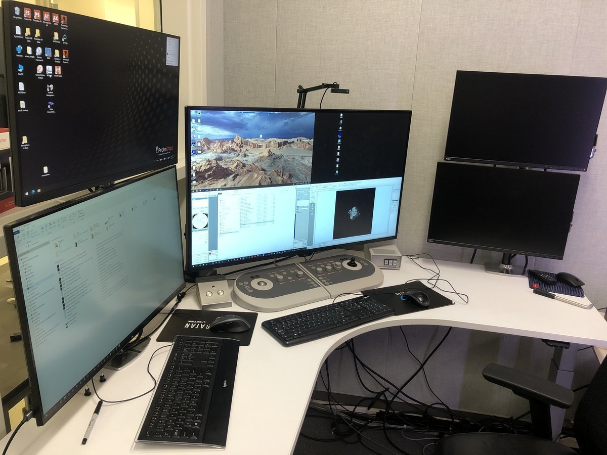
Workstation layout:
| Monitor | Software | Purpose |
|---|---|---|
| Bottom left | TEMUI | Microscope control, vacuum, alignments |
| Bottom right | Velox | Live imaging, acquisition |
| Top left | Probe Corrector S-CORR | Aberration measurement & correction |
| Top right | Velox image gallery | Captured images from Velox |
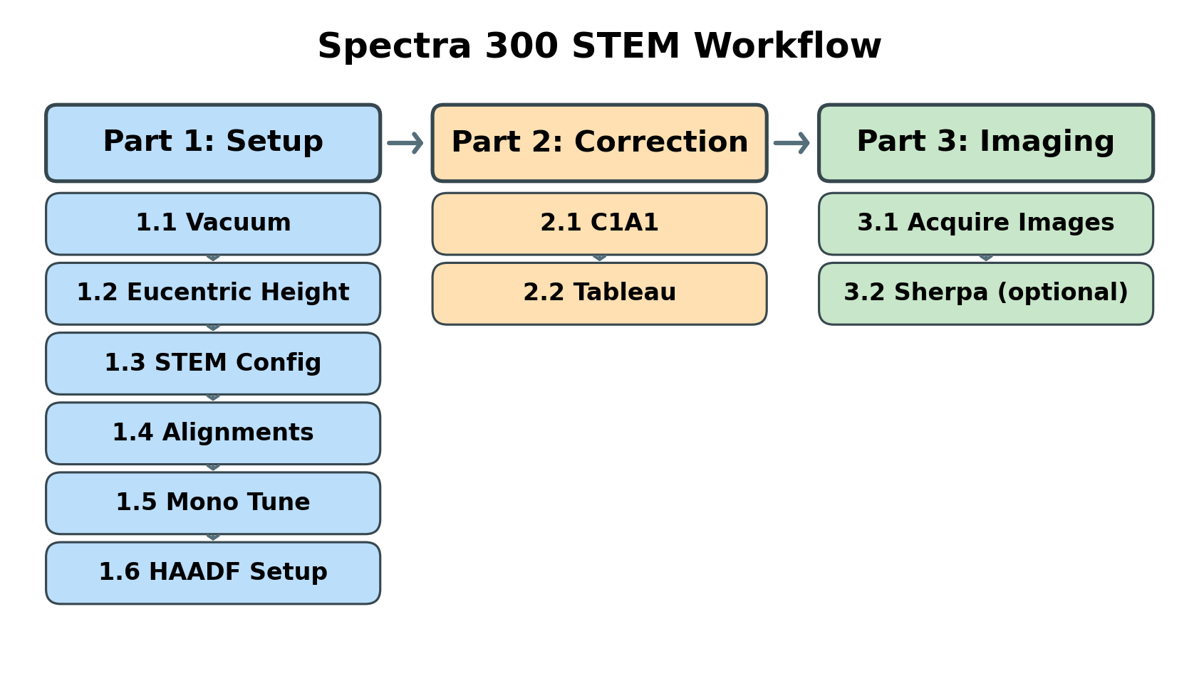
Overview
This guide covers three main phases:
| Phase | Procedures | Time |
|---|---|---|
| Part 1: Setup & Alignment | Vacuum check, eucentric height, STEM mode configuration, direct alignments, monochromator tune, HAADF setup | 5-10 min |
| Part 2: Probe Correction | Correct aberrations (C1A1, Tableau) to achieve sub-angstrom probe | 10-15 min |
| Part 3: Imaging | Image acquisition, Sherpa fine-tuning (optional), load your own sample | varies |
| Part 4: End session | Reload standard sample, pre-departure checklist | 5 min |
Part 1: Setup & Alignment
1.1 Vacuum check
Before imaging, verify that the vacuum system is ready and the column valves can be safely opened. Poor vacuum conditions can damage the electron source and contaminate the sample.
-
Check vacuum status
-
In
TEMUI, openSetuptab. -
Locate vacuum status panel. Status shows “All Vacuum (Closed)” and
Col. Valves Closedbutton is yellow.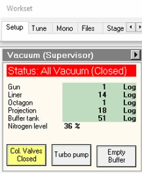
-
-
Verify vacuum pressure
-
Check vacuum pressure values on the log scale (lower = better):
Gauge Typical Log Value Notes Gun 1 Critical for source lifetime Liner 14 Column vacuum Octagon 1 Sample area Projection 19-21 Below sample Buffer tank 41-51 Empty if above 51 -
If buffer tank pressure is above 51, click
Empty Buffer.- Pumps cycle audibly.
-
Wait for value to decrease before proceeding.
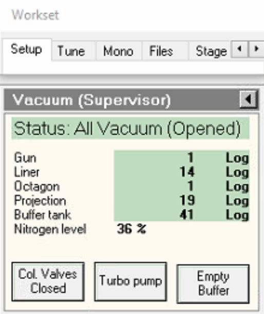
-
-
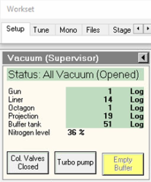
Open column valves
-
Click
Col Valves Closedbutton.- Status changes to “All Vacuum (Opened)”.
NOTE: The system only allows opening if vacuum levels are acceptable. Once opened, the electron beam path is clear from gun to sample.
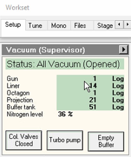
-
1.2 Check convergence angle
For this guide, we use a convergence angle of 30.0 mrad.
- In
TEMUI, navigate to theTunetab, then selectAperture. - Set Condenser 1, Condenser 2, and Condenser 3 to
2000,70, and1000.
NOTE: These aperture values determine the convergence angle. For example, setting Condenser 2 to
50instead of70gives a convergence angle of 21.5 mrad. A smaller aperture restricts the beam to a narrower range of incident angles, blocking higher-angle electrons.
1.3 Find eucentric height
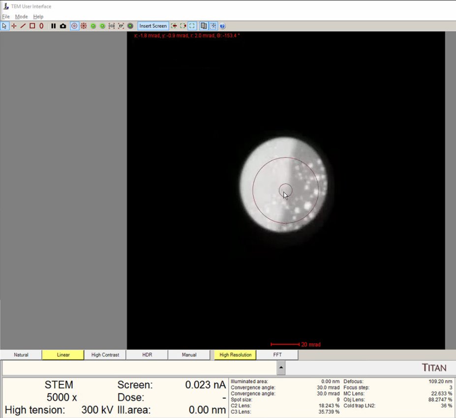
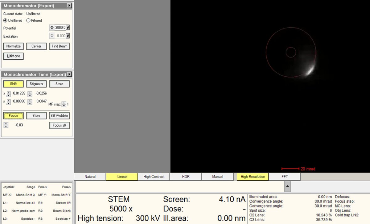
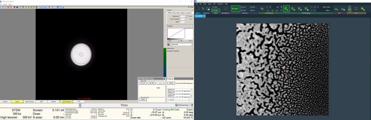
Complete eucentric height alignment after loading each sample and before imaging. Do not skip this step. At eucentric height, the sample remains stationary when tilted. This is essential for accurate imaging and tomography. The ronchigram “blow-up” method provides a quick way to find this position.
-
View ronchigram
-
Verify the
Diffractionbutton is pressed on the hand panel with the red light turned on.NOTE: The ronchigram is the diffraction pattern formed when the convergent probe is stationary. When defocused, it contains shadow images of sample features, making structure visible during z-height adjustment.
-
In
TEMUI, view the ronchigram in the main display.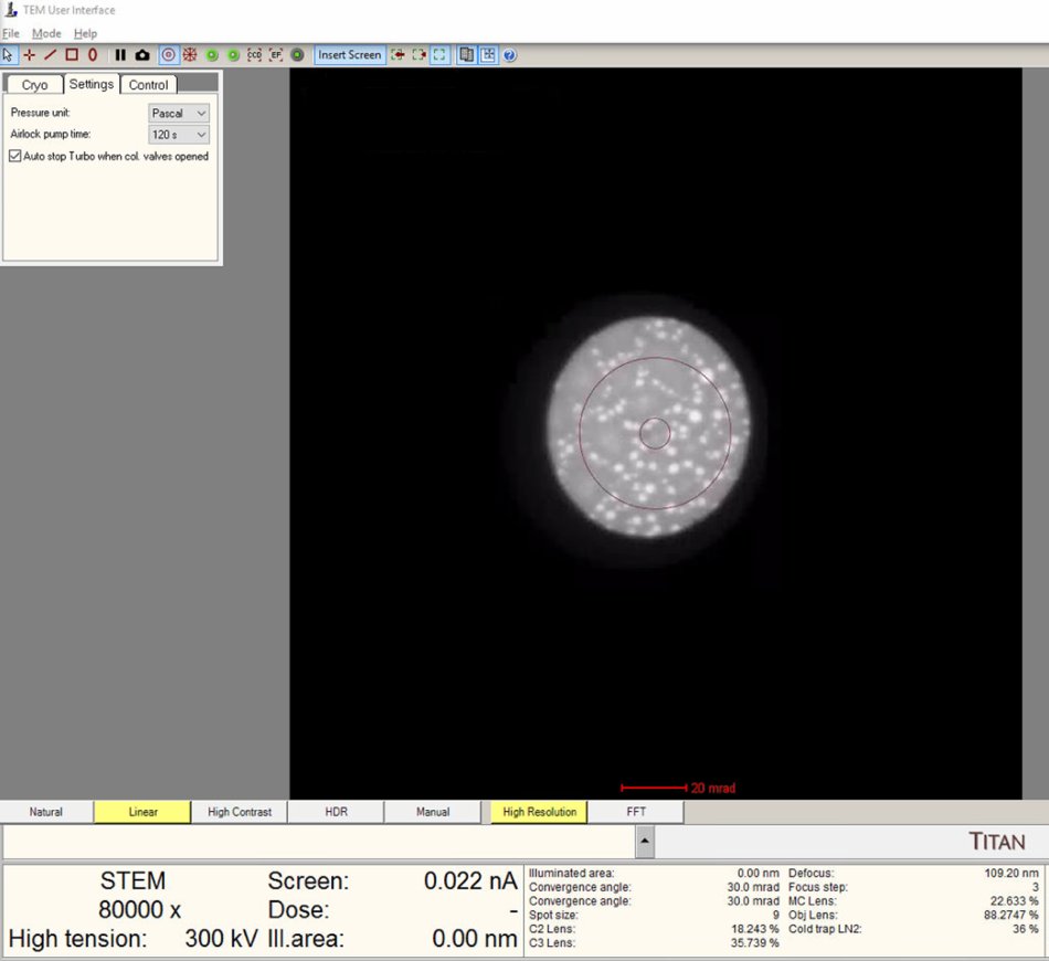
-
Position probe on a sample region that scatters electrons (not over a hole or vacuum).
-
-
Adjust z-axis to find blow-up point
-
Lower magnification to 5,000x. A wider field of view makes ronchigram changes easier to observe.
-
Find a region where there is a sharp contrast at a boundary, as shown in the following image.
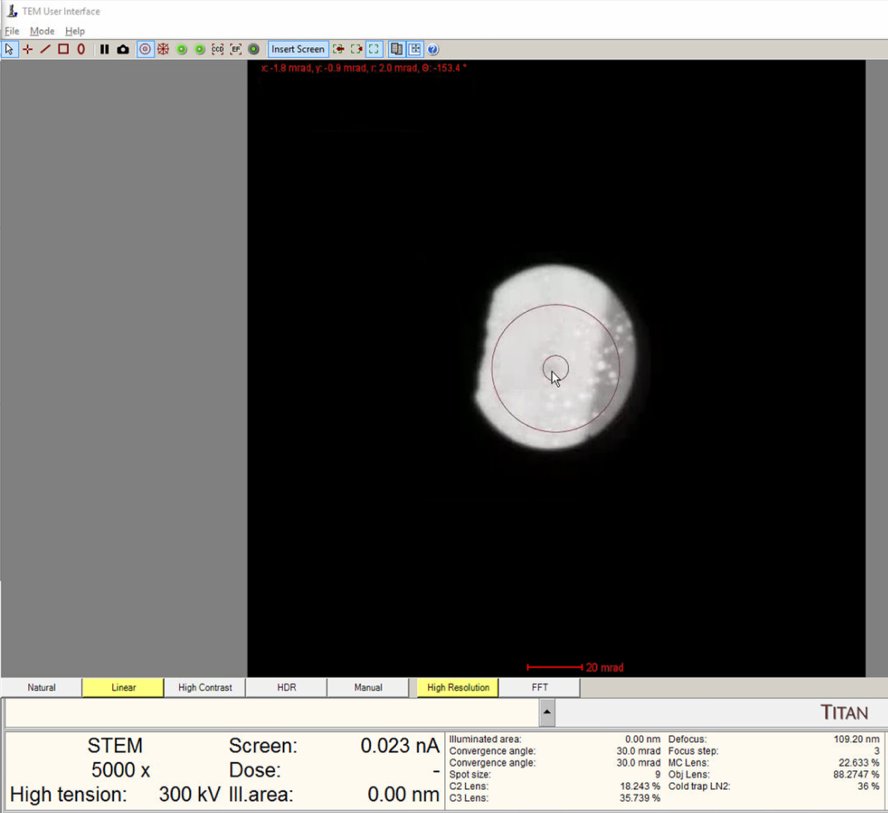
-
Use z-axis buttons on hand panel to move stage up or down.
- Buttons are pressure sensitive: press harder for faster movement.
- Start with gentle presses for fine control.
- Notice that as you adjust the z-axis, the ROI also shifts. Use the joystick to remain on the sharp contrast boundary region.
-
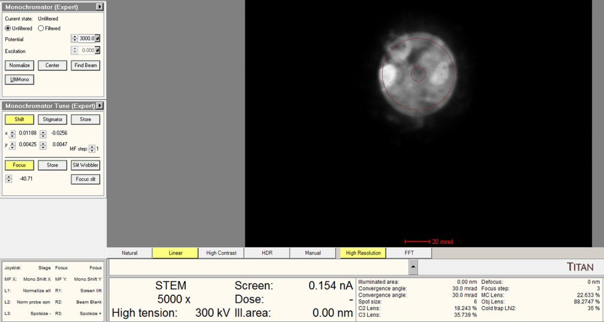
Watch the ronchigram while adjusting z-height. The pattern “zooms” in or out as the sample moves through focus.
-
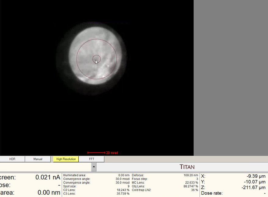
Continue adjusting. The ronchigram expands when approaching eucentric height, also referred to as the “blow-up” point.
-
Find the “blow-up” point where the ronchigram appears infinitely magnified: shadow image features expand until they fill the entire display.
- If the ronchigram starts shrinking again, reverse direction.
-
1.4 STEM mode configuration
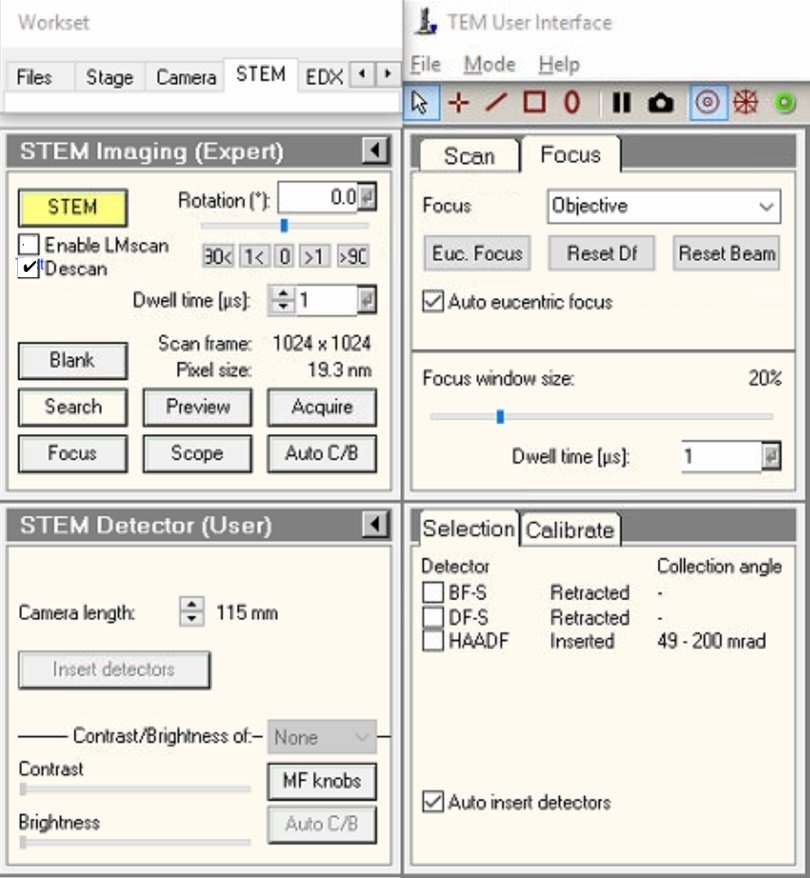
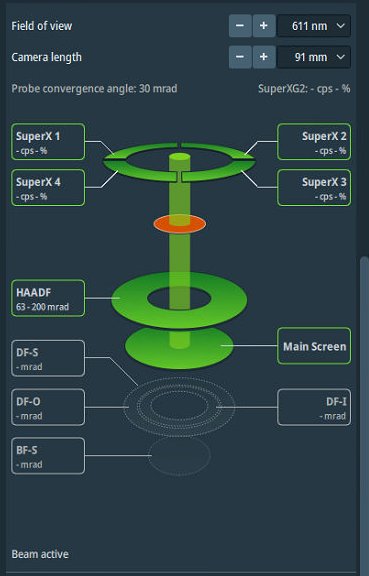
Before performing alignments, configure the STEM imaging parameters and verify detector settings.
-
Enable descan
-
In
TEMUI, locate theSTEM Imaging (Expert)panel. -
Enable
Descancheckbox.NOTE: Descan compensates for beam movement during scanning, keeping the diffraction pattern stationary on the detector.
-
-
Verify HAADF is retracted
-
Locate the
Selectionpanel. -
Verify detector states:
- BF-S (Bright Field): Retracted
- DF-S (Dark Field): Retracted
- HAADF: Retracted
-
Toggle
HAADFcheckbox on then off to confirm retracted state.NOTE: HAADF must be retracted during ronchigram alignment. The HAADF is a ring-shaped detector with a central hole. If inserted, high-angle electrons hit the ring instead of the camera below, blocking part of the ronchigram.
-
-
Set detector layout in Velox
-
Open
Veloxacquisition software. -
Open detector layout display.
-
Set camera length to 91 mm.
NOTE: Camera length determines detector collection angles. The layout display shows the angular ranges for each detector.
-
-
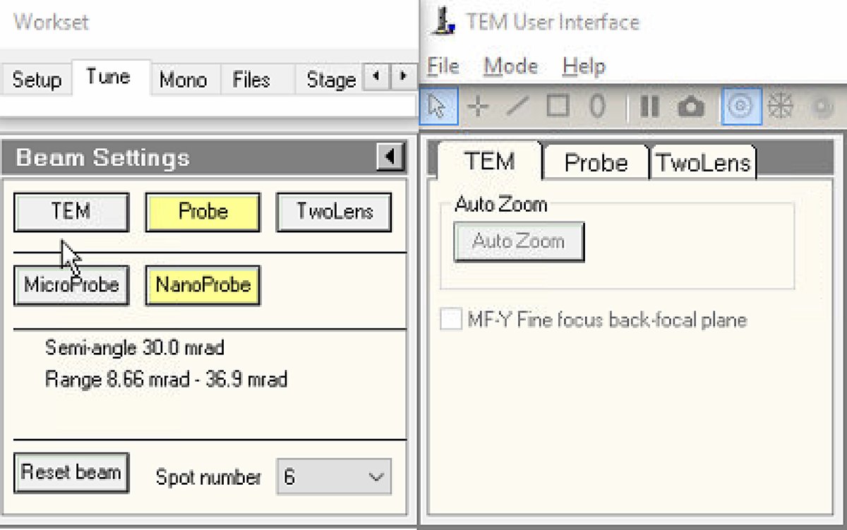
Configure beam settings
-
In
TEMUI, go to theTunetab and locate theBeam Settingspanel. -
Select
Probemode.- Button is highlighted yellow when active.
-
Select
NanoProbemode. -
Set spot number to 6.
NOTE: NanoProbe provides a smaller, more coherent probe than MicroProbe. Lower spot numbers produce smaller probes with lower current; higher numbers produce larger probes with more current.
TODO: Verify spot number convention for Spectra 300. On some Thermo Fisher systems, it is the opposite (spot 1 = most current).
-
1.5 Direct alignments
The basic alignments center the electron beam and align it through the optical column. Proper alignment is essential for optimal resolution and probe symmetry.
-
Set magnification and open Direct Alignments
-
Set magnification to 200-300kX using the magnification knob.
-
In
TEMUI, navigate toTunetab, thenDirect Alignments. This panel provides access to all fundamental beam alignment procedures. -
Select
Diffraction Shift and Focus alignmentto begin.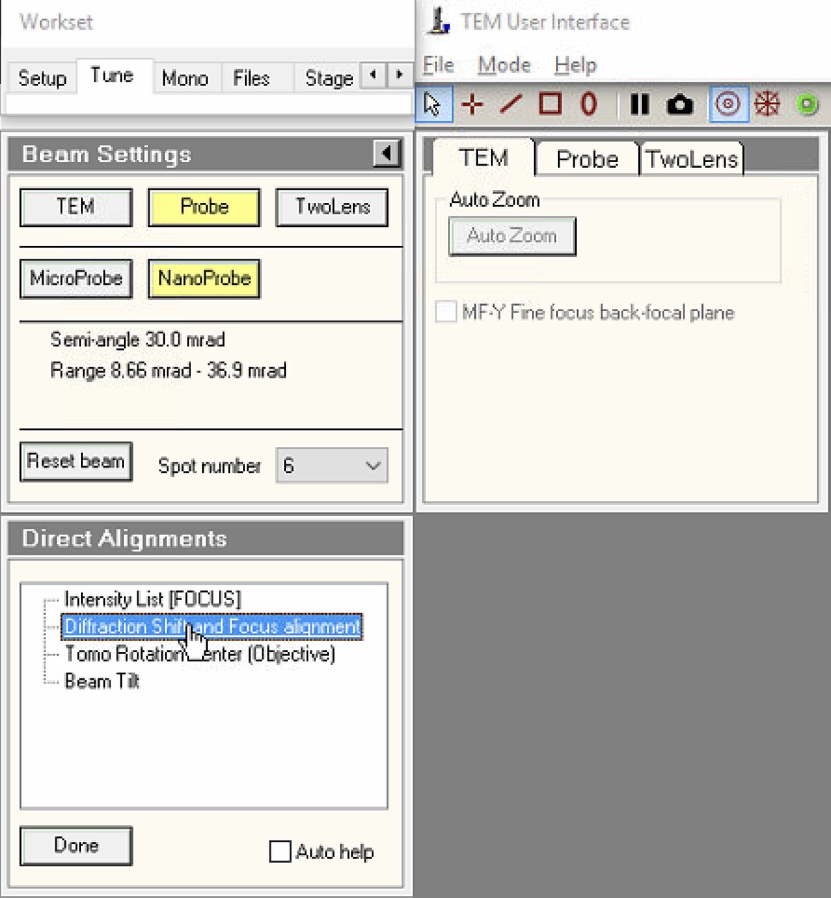
-
-
Center ronchigram
-
Observe the ronchigram position on the display. If the ronchigram is shifted from center, use the
mulXYknobs to bring it back.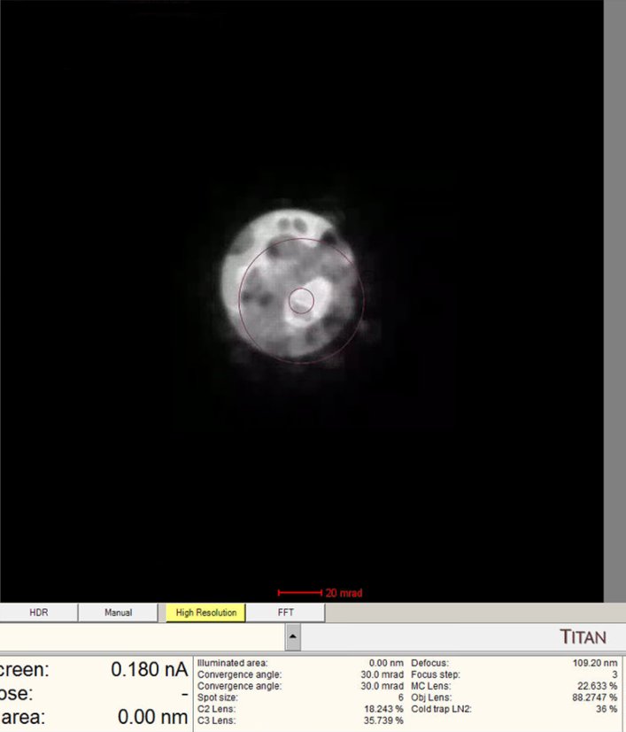
-
The
mulXYknobs now control diffraction shift. Adjust until the ronchigram is centered.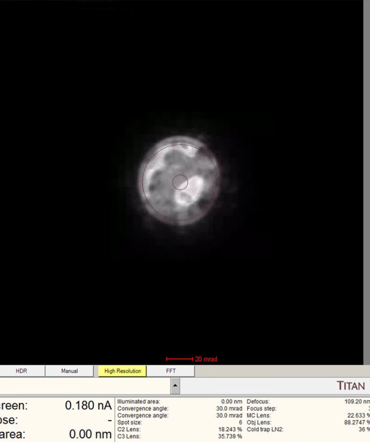
-
-
Reset STEM AutoTuning
-
In the quick dropdown menu, select
STEM AutoTuning. This panel stores automatic alignment adjustments from previous sessions. -
Click
Resetunder Settings to clear stored values. This establishes a known baseline. Previous user adjustments persist and interfere with fresh alignments if not reset.
-
-
Switch to probe image mode
-
Press the
Diffractionbutton on the hand panel to enter probe image mode (STEM scanning). The red light should turn off once pressed.No beam found? In the following step you will click
Beam Shiftand adjust themulXYknobs. Watch the screen current: it changes from 0.000 nA to 0.001 nA, etc. This means you are shifting the beam position near the screen. You will see dim light coming from the edges. Press theFineandCoarsebuttons to adjust the sensitivity of themulXYknobs.Still can’t find the beam at all? Try temporarily increasing the C2 aperture from
70to150in theAperturespanel. The larger aperture lets more electrons through, making the beam much easier to locate. Once you find and center the beam, switch back to70before continuing.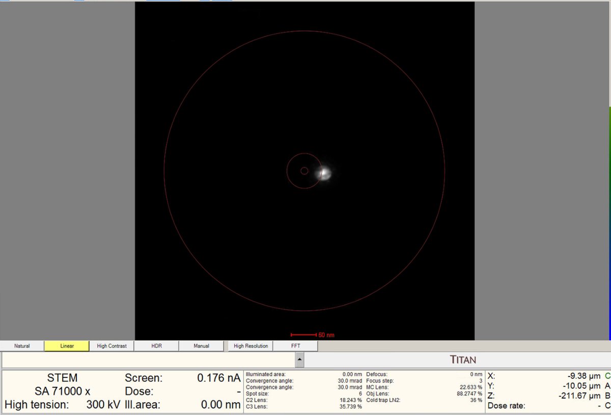
Diffraction mode vs. Probe image mode
Mode Probe Display Diffraction mode Stationary Ronchigram - diffraction pattern from convergent probe Probe image mode Scanning STEM image - probe scans to build up image pixel by pixel The
Diffractionbutton on the hand panel toggles between these two modes.
-
-
Align beam shift
-
Click on
Beam shiftin the Direct Alignments panel. ThemulXYknobs now control alignment beam shift. -
Use the
mulXYknobs to center the beam on the screen. The beam responds smoothly to knob movements. If the beam moves too quickly, pressFineon the hand panel to reduce sensitivity. -
Important: If the beam is lost after clicking beam shift, reduce magnification until the beam is visible, center using the
mulXYknobs. -
Click
Doneonce the beam is properly centered.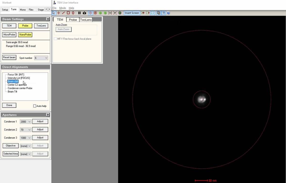
-
-
Center C2 aperture
-
Select
Center C2 aperturefrom the alignment options. The system oscillates the C2 lens, causing the beam to expand and contract rhythmically. -
Watch the beam movement carefully. The beam pulses in and out. The goal is to make this expansion/contraction perfectly concentric (no lateral movement).
-
Use the
mulXYknobs to adjust the aperture position. -
Click
Donewhen the movement is concentric.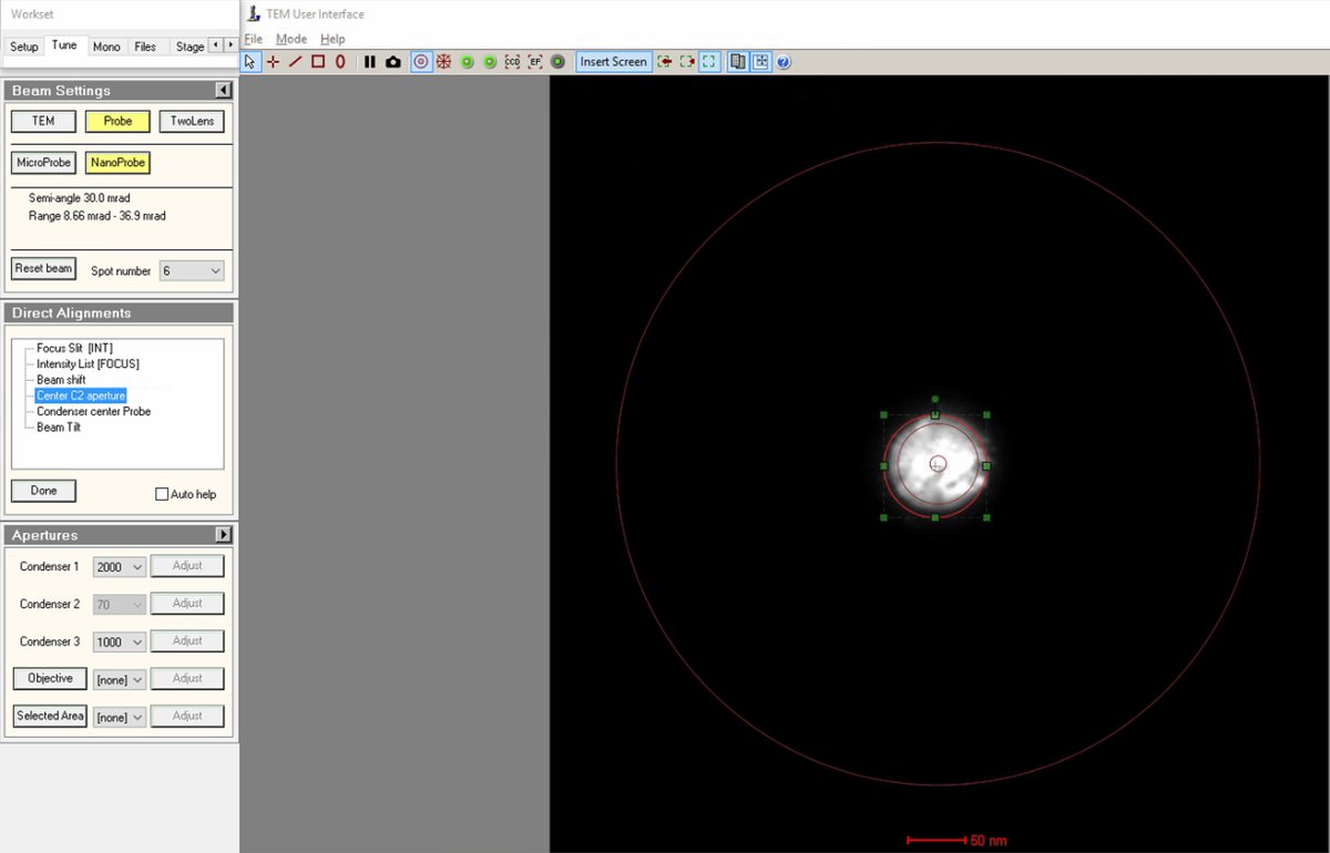
-
-
Align beam tilt
-
Select
Beam Tiltfrom the alignment options. This alignment minimizes the lateral shift of the beam when tilting. -
Use the
mulXYknobs to minimize lateral movement of the beam. When properly aligned, the beam changes angle without shifting position. -
Reduce the lateral x and y movements as much as possible using the
mulXYknobs. -
Click
Doneonce the lateral movement is minimized.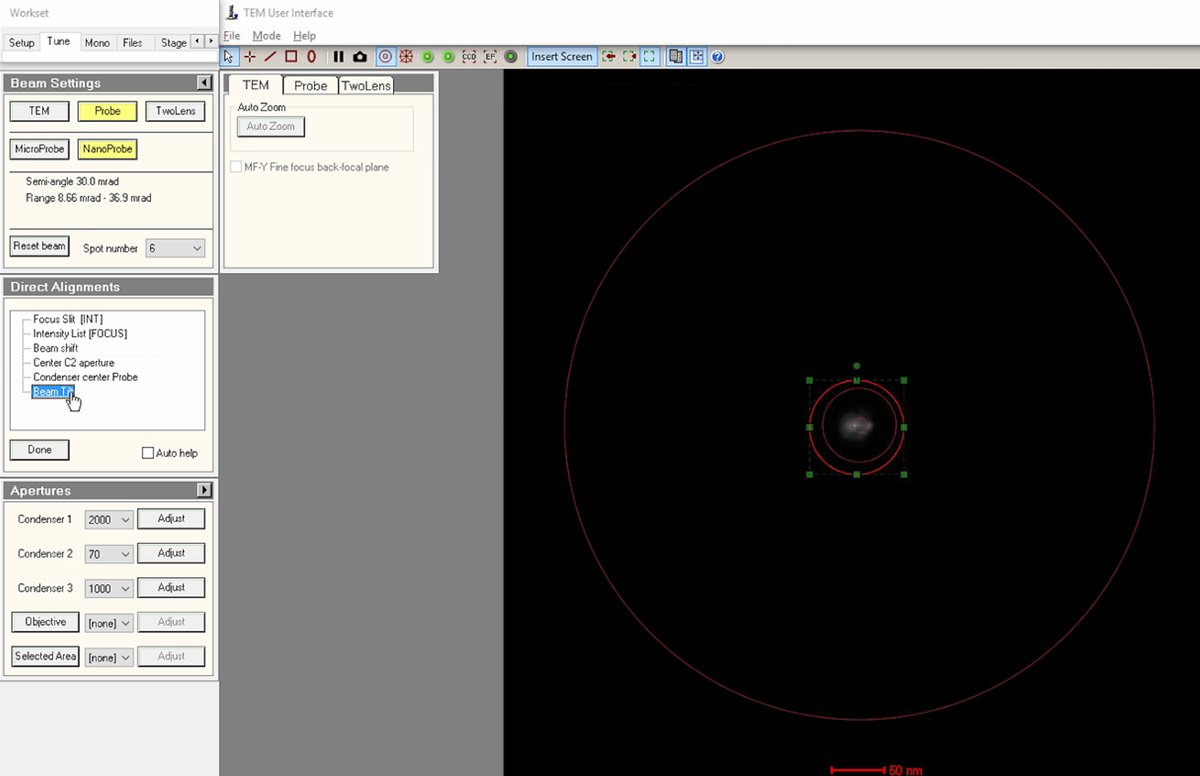
-
-
Verify final diffraction shift
-
Press the
Diffractionbutton on the hand panel to switch back to diffraction mode (view the ronchigram). The red light should now be on. -
Return to
Diffraction Shift and Focus alignmentfor a final centering check. -
Use
mulXYto center the ronchigram precisely on the display. Centering confirms the beam is on the optical axis. -
Click
Doneto complete the direct alignments.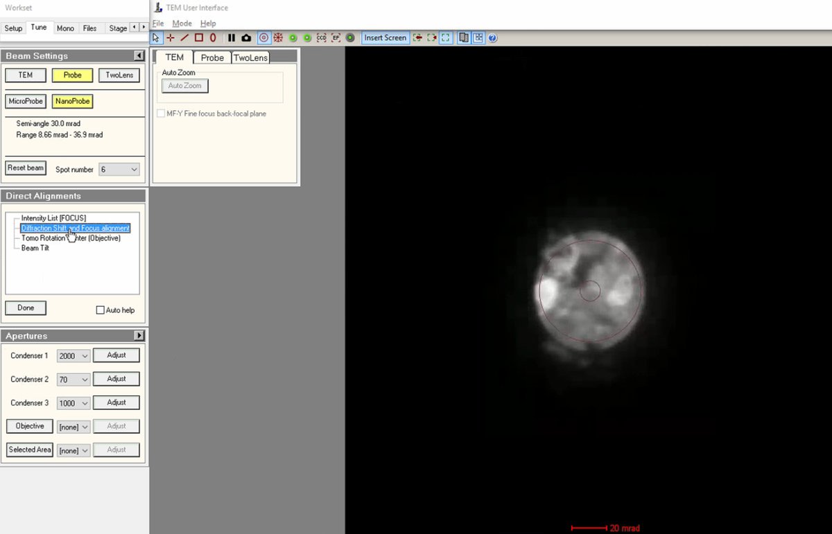
-
Note: Mode changes (diffraction ↔ probe image, TEM ↔ STEM) disable descan. Re-enable descan after each mode switch. If the image looks distorted, verify
Descanis enabled inSTEM Imaging (Expert).
1.6 Monochromator tune
Before proceeding to probe correction, check that the monochromator is properly aligned and not partially blocking the beam. The monochromator selects a narrow energy spread from the electron source, improving resolution but reducing beam current.
-
Open Monochromator Tune
-
In
TEMUI, go to theMonotab and locate theMonochromator Tune (Expert)panel. This panel provides controls for adjusting the monochromator position and focus. -
Click on both
ShiftandFocusbuttons to enable adjustment mode. At this point, the intensity knob controls monochromator focus and themulXYknobs control monochromator shift.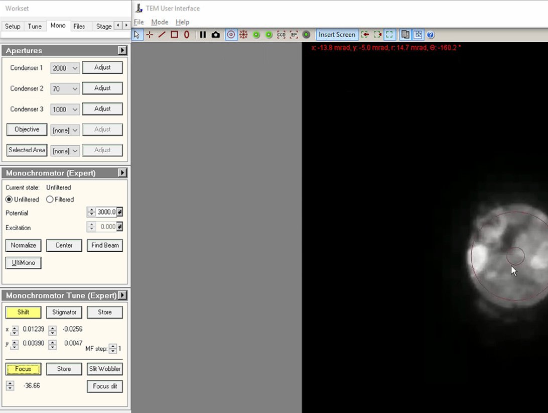
-
-
Adjust focus
-
Adjust the intensity knob to bring the Focus value close to 0. As the monofocus approaches zero, the screen current increases because more electrons pass through the monochromator slit.
-
While adjusting Focus toward 0, also adjust the
mulXYknobs to ensure the beam isn’t blocked. The screen current inTEMUIshould be above 15 nA when focus is near zero.No beam visible? Click
Linearin the detector settings to switch from log to linear display mode. If the beam is still missing, return to the initial focus value and slowly bring it back toward 0 while adjustingmulXY, as in the Beam Shift alignment. -
Watch the current readout while adjusting.
-
-
Center and adjust current
-
Adjust the
mulXYknobs to center the beam through the monochromator.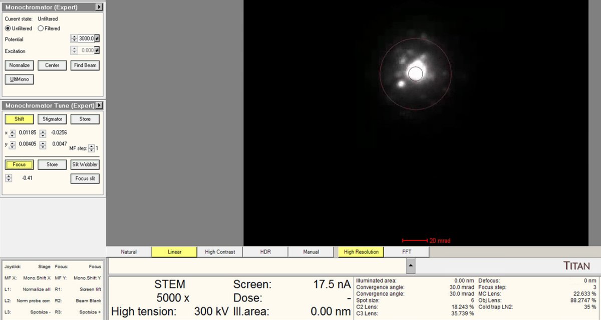
-
Use the intensity knob to achieve the target beam current (~0.150 nA for high-resolution STEM).
-
-
Deselect Shift and Focus
- Click
Shiftagain to deselect both buttons (they toggle together). - This returns the intensity knob and
mulXYknobs to their normal functions. Verify the current readout shows the target value before proceeding.
- Click
-
Re-verify eucentric height
- Use the z-axis controls to return to the “blow-up” point (eucentric height). Monochromator adjustments affect focus; re-verify eucentric height.
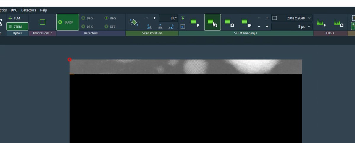
1.7 HAADF imaging setup
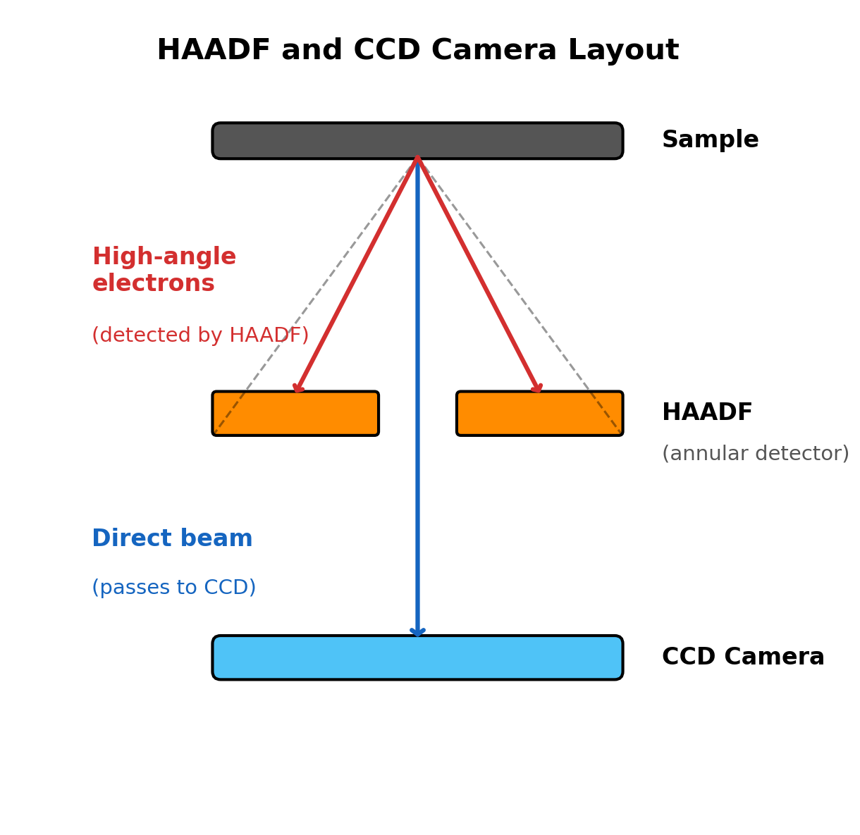
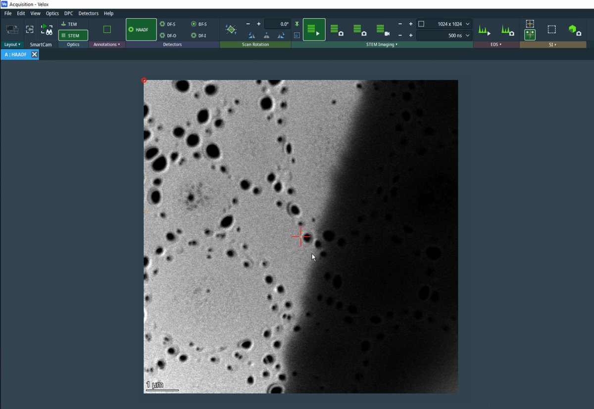
Before running aberration correction, set up HAADF (High-Angle Annular Dark Field) imaging to view the sample and find a suitable region. HAADF provides Z-contrast imaging where heavier atoms appear brighter.
-
Switch to HAADF
-
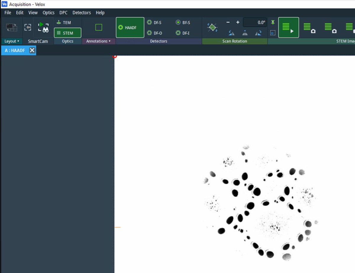
In the
Veloxacquisition software, clickSTEMto enter STEM mode, -
Click
HAADF. This automatically inserts the HAADF detector. -
Verify in
TEMUIthat the HAADF detector shows “Inserted” status with the correct collection angle (63-200 mrad).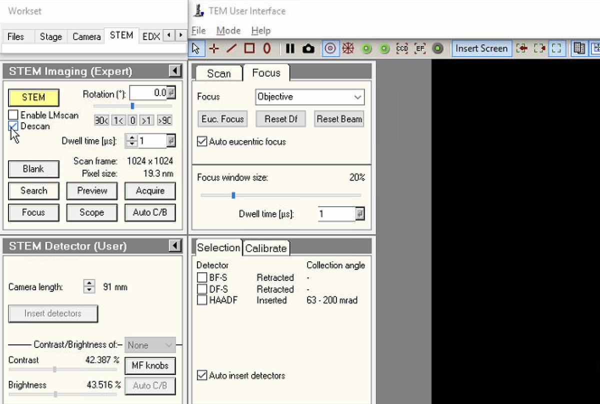
-
-
Verify Descan is enabled
- In
TEMUI, go toSTEM Imaging (Expert)and verifyDescanis enabled. Mode changes disable descan; re-enable after switching modes.
- In
-
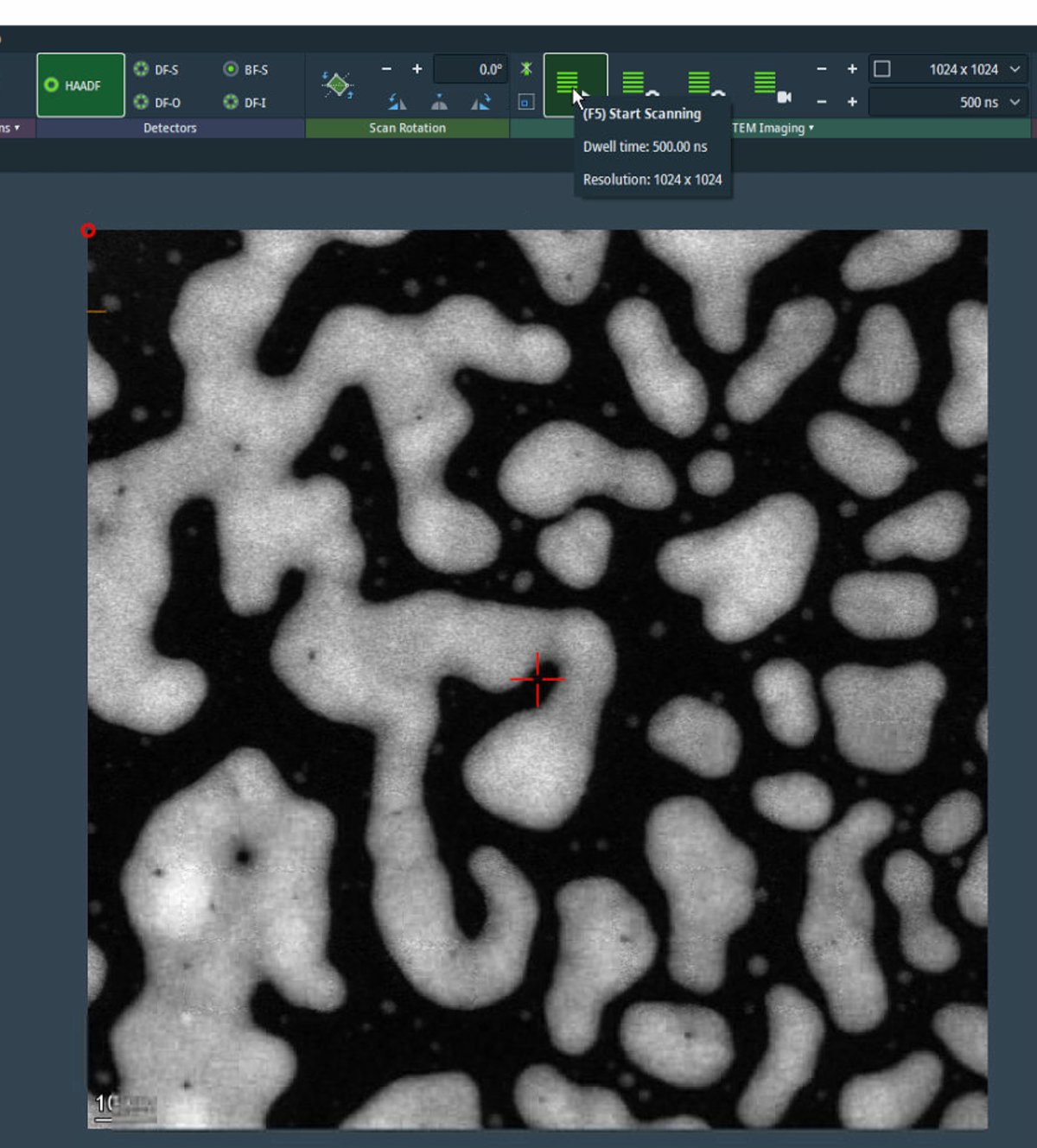
Start live scanning
-
Click the play button in
Veloxto start live scanning. -
The image is saturated (all white) initially. Detector signal adjustment follows in the next step.
-
-
Adjust detector signal
-
In
Velox, clickScope toolto enable signal adjustment. -
Adjust
GainandOffsetso the signal does not go above the dotted red lines.Signal math: Display = (Gain × Signal) + Offset
- Gain (= Contrast): Multiplier that stretches the signal. 100% = no change, 200% = double the contrast
- Offset (= Bias/Brightness): Shifts the baseline as a percentage of the display range
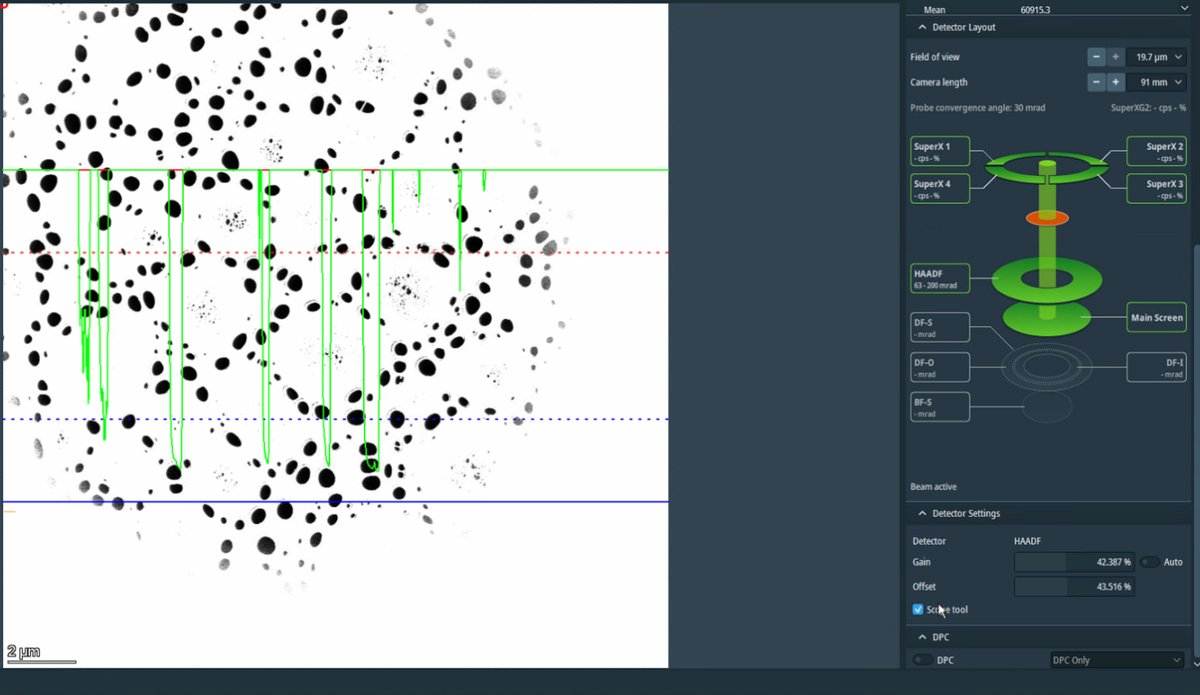
-
If the signal is clipping at zero (bottom of display), increase
Offsetto shift the signal up.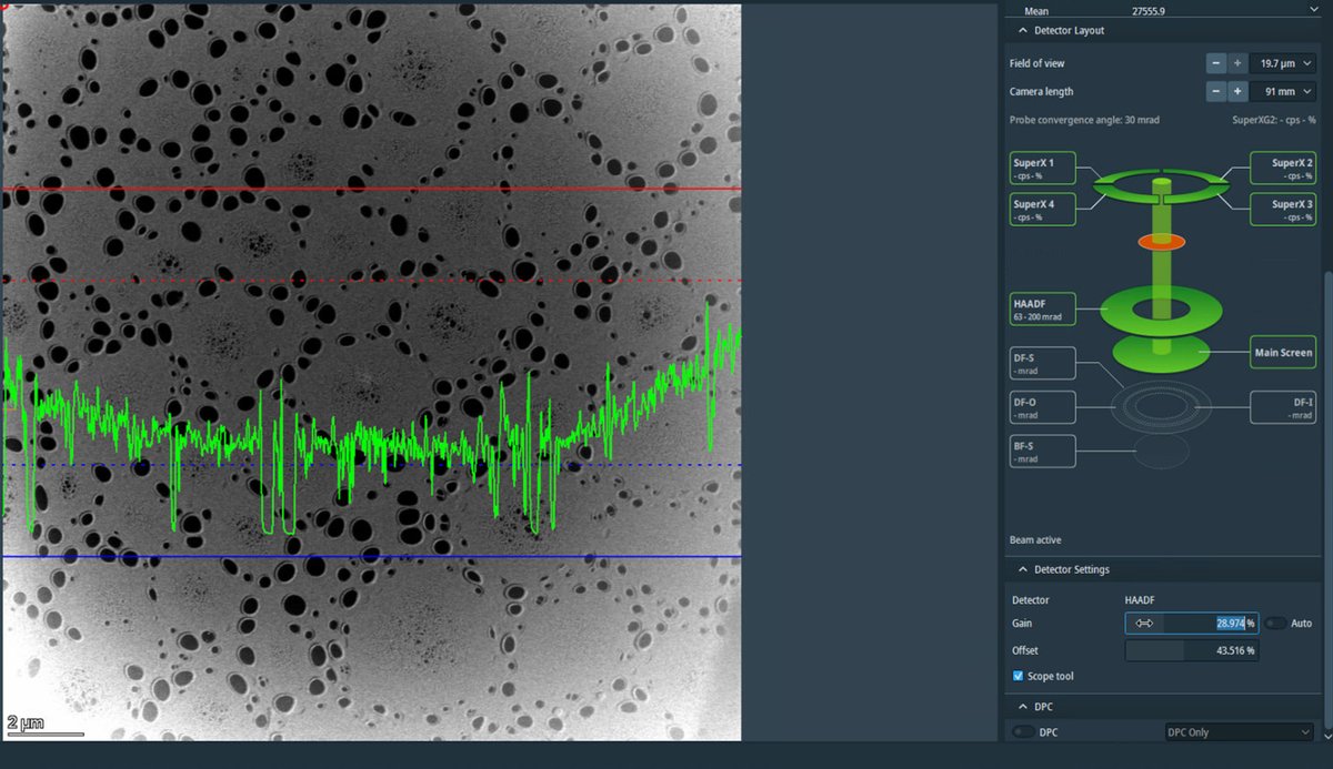
-
Adjust the magnification to ~20,000x using the magnification knob. Once adjusted, uncheck
Scope toolto turn it off.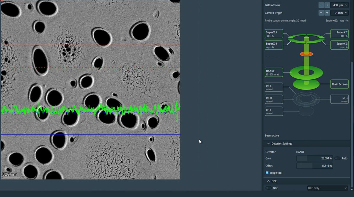
-
-
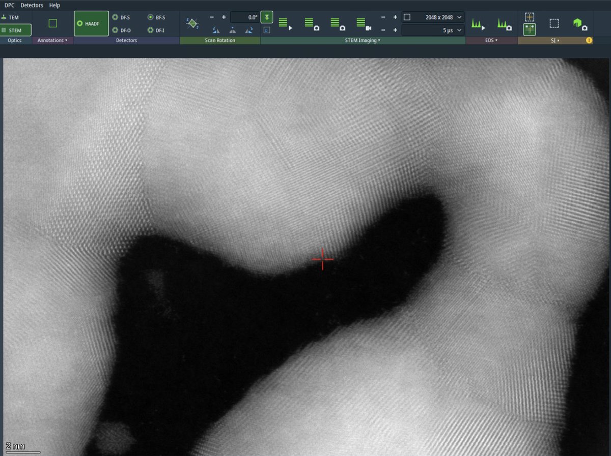
Find sample boundary
-
Reduce magnification to ~10,000x and navigate with the joystick to find a suitable region.
-
Locate a boundary region with particles at the edge of a support film, with vacuum visible.
-
This type of region provides excellent contrast for aberration correction.
-
-
Adjust focus
-
Once a suitable boundary is found, increase magnification to ~160,000x. Alternate between magnification and z-axis adjustments until focus is sharp.
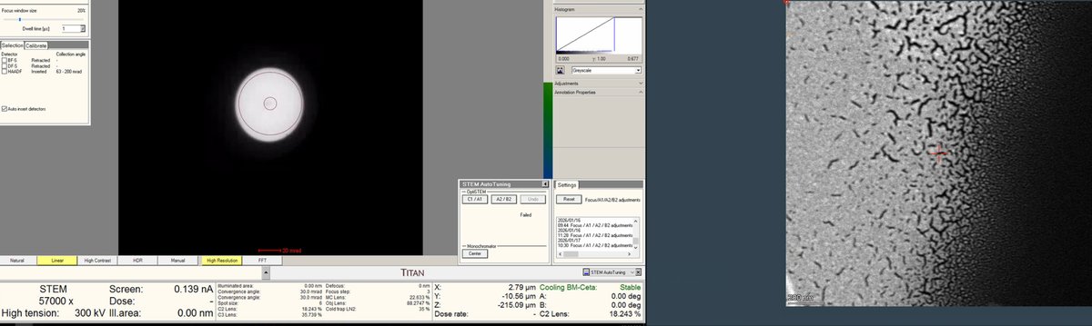
-
Adjust the z-axis while watching the HAADF image. Features become sharper as focus is approached.
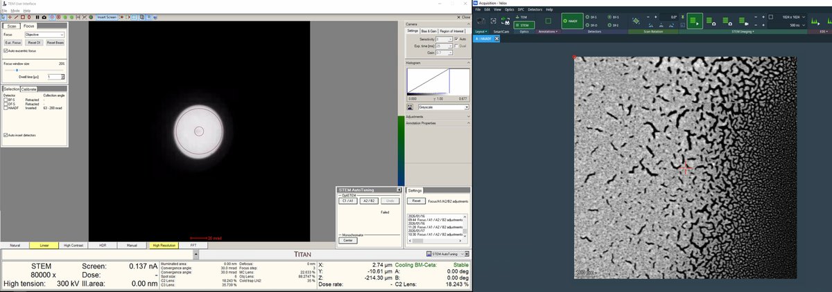
-
Continue adjusting magnification and z-axis.
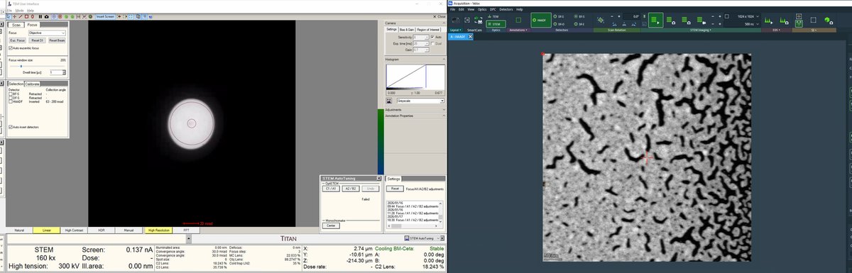
-
Finalize the position with sharp features and distributed particle sizes.
Distributed particles are important for aberration measurement. Aberrations vary with position relative to the optical axis (e.g., coma increases further from center). The correction algorithm requires ronchigram data from multiple positions to accurately fit the aberration coefficients.
-
Part 2: Probe Correction
Before starting probe correction, retract the HAADF detector. C1A1 and Tableau both analyze the ronchigram, and the HAADF ring blocks high-angle electrons from reaching the camera below. In TEMUI, verify the HAADF detector shows “Retracted” status.
TODO: Confirm with staff whether HAADF must be retracted for C1A1/Tableau on Spectra 300 S-CORR.
Aberrations distort the electron probe and degrade image resolution. The goal of probe correction is to achieve a flat, aberration-free ronchigram. The figure below shows how individual aberrations affect the ronchigram appearance:
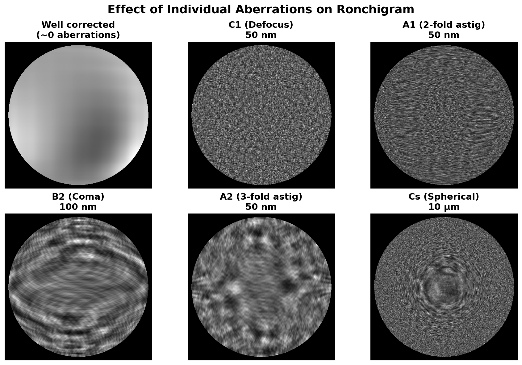
Interactive demo: Explore how aberrations affect the ronchigram at bobleesj.github.io/electron-microscopy-website/ronchigram
Probe correction uses two tools in the Probe Corrector S-CORR software:
| Tool | What it corrects | How it works |
|---|---|---|
| C1A1 | First-order: defocus (C1) and 2-fold astigmatism (A1) | Continuous ronchigram measurement; click buttons to apply |
| Tableau | Higher-order: A2, B2, C3, S3, A3 | Single measurement sequence with beam tilts; then apply |
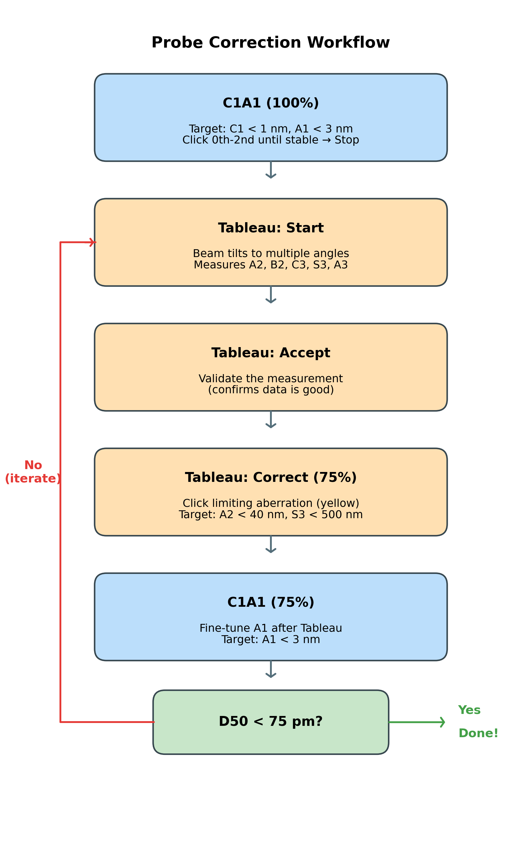
The correction workflow:
The following workflow is covered in this section. Follow the steps below, then use this diagram as a quick reference:
2.1 C1A1 correction
C1A1 corrects first-order aberrations: defocus (C1) and 2-fold astigmatism (A1). These are the dominant aberrations that must be corrected before higher-order Tableau measurement. The C1A1 procedure analyzes the ronchigram to measure and correct these aberrations iteratively.
-
Open Probe Corrector
-
On the top left monitor, open the
Probe Corrector S-CORRsoftware (main interface for aberration measurement and correction). -
Check the mode indicator in the top right. Verify it shows
STEM@300KV: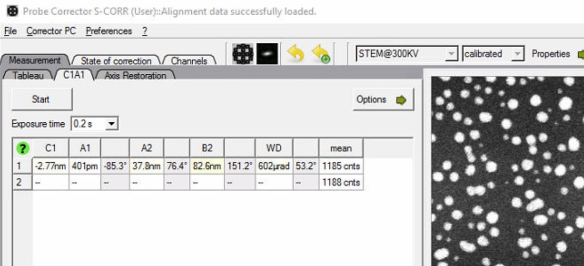
-
If
MC_STEM@300KVappears instead, the system is in monochromated STEM mode. Follow the steps below to reset to standard STEM mode. IfSTEM@300KVis displayed, skip ahead to “Configure C1A1 options.”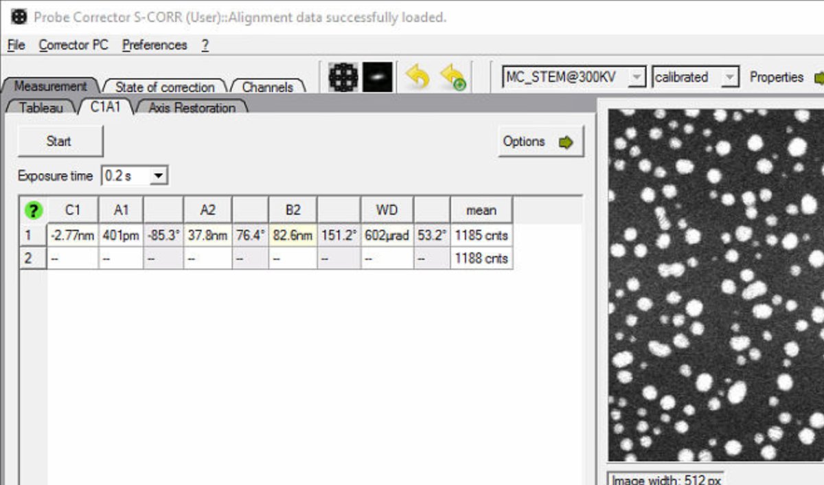
-
To reset, in TEMUI go to
Mono, then openMonochromator (Expert)and clickFilter: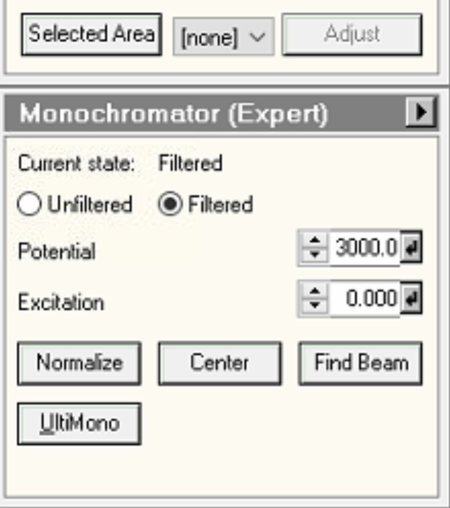
-
Then click
Unfilterto reset to standard STEM mode: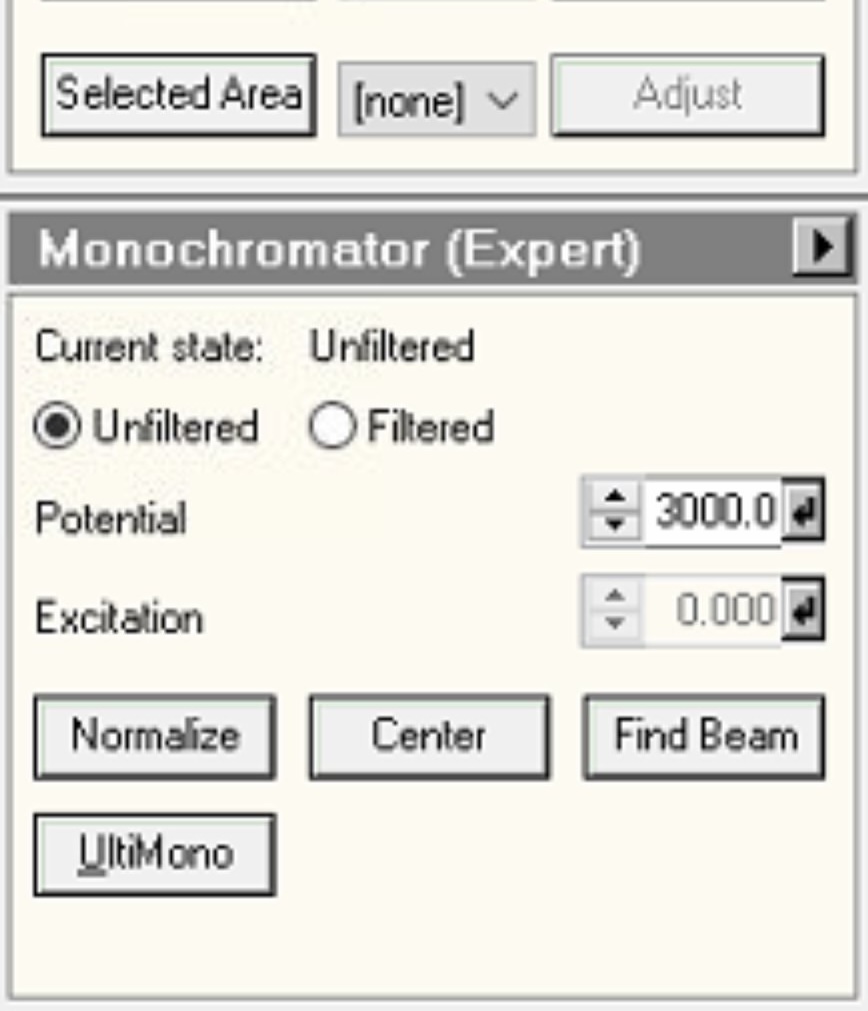
-
-
Configure C1A1 options
-
In the Probe Corrector software, click
Optionsto expand the configuration panel: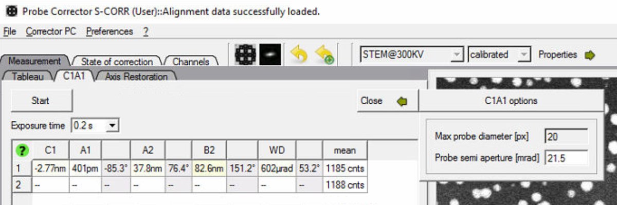
-
Set
Probe semi apertureto 30 mrad: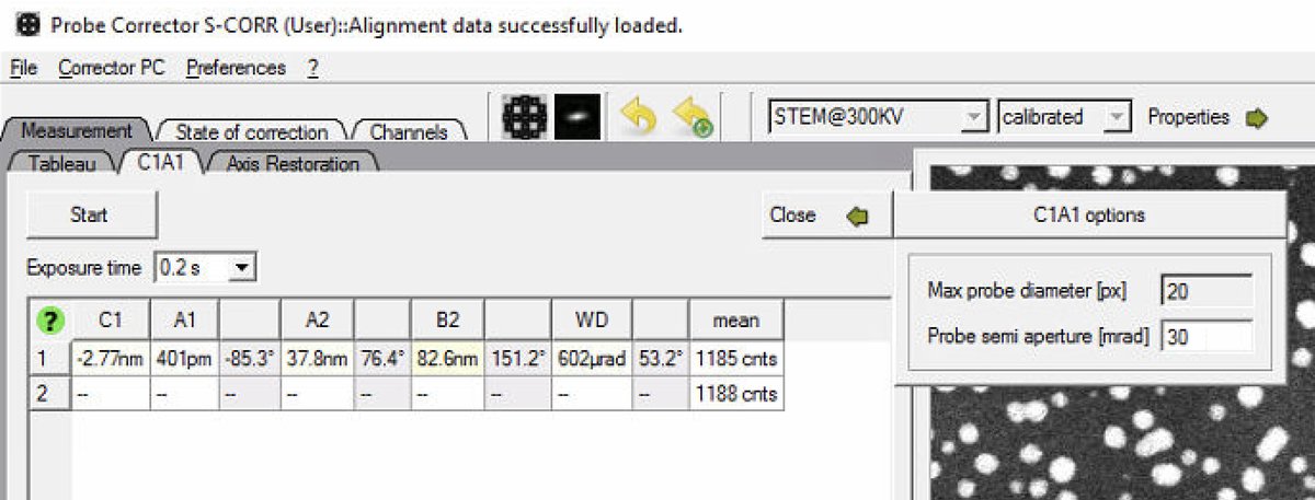
-
-
Switch to diffraction mode
-
Stop live scanning in
Veloxby clicking the play button, then ensureDiffractionmode is on on the hand panel. C1A1 analyzes the ronchigram, so diffraction mode (stationary probe) is required, not probe image mode (scanning):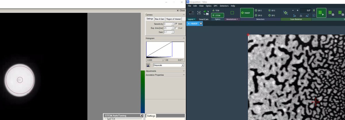
-
Click the
Beam Blankbutton to unblank the beam. Stopping the scan automatically blanks the beam. The Probe Corrector software requires an unblanked beam to read the ronchigram: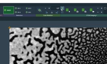
-
-
Run C1A1
-
Go to the
C1A1tab in theProbe Correctorsoftware. Before clicking Start, verify the ronchigram is visible on the left monitor: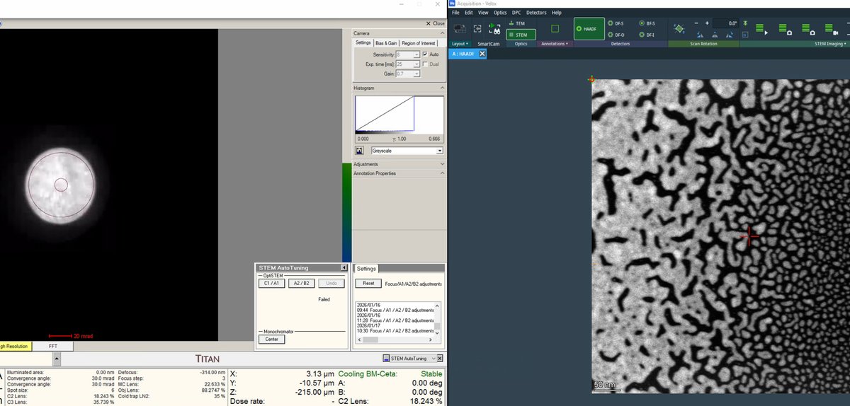
-
Click
Startto begin aberration measurement. The software continuously analyzes the ronchigram and displays measured aberration values (C1, A1, A2, B2, WD) in the table. -
Set Auto correct to 100% for the first iteration.
-
Click
0th-2ndto apply corrections for all first and second order aberrations.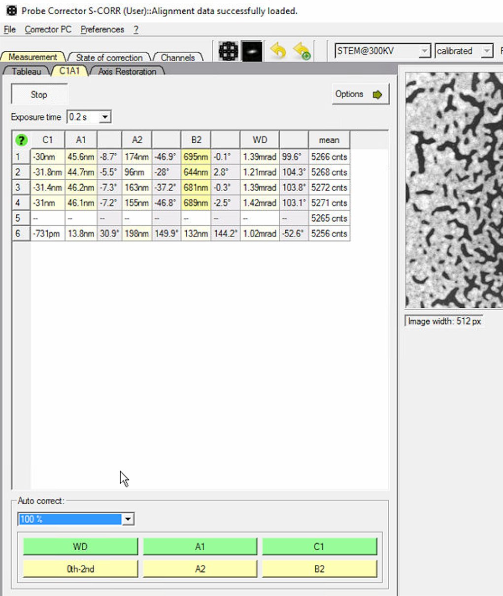
-
-
Iterate C1A1
-
Click
0th-2ndrepeatedly to apply corrections. Each row represents one measurement cycle. Watch the aberration values decrease with each iteration.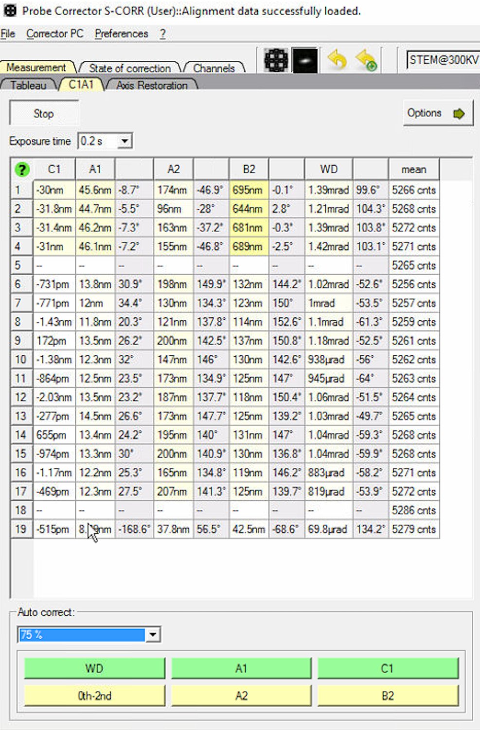
-
Reduce the Auto correct percentage to 75% after several iterations (typically 3 to 5) to prevent overcorrection.
If A1 is still high but other values are good, click
A1specifically to correct only astigmatism.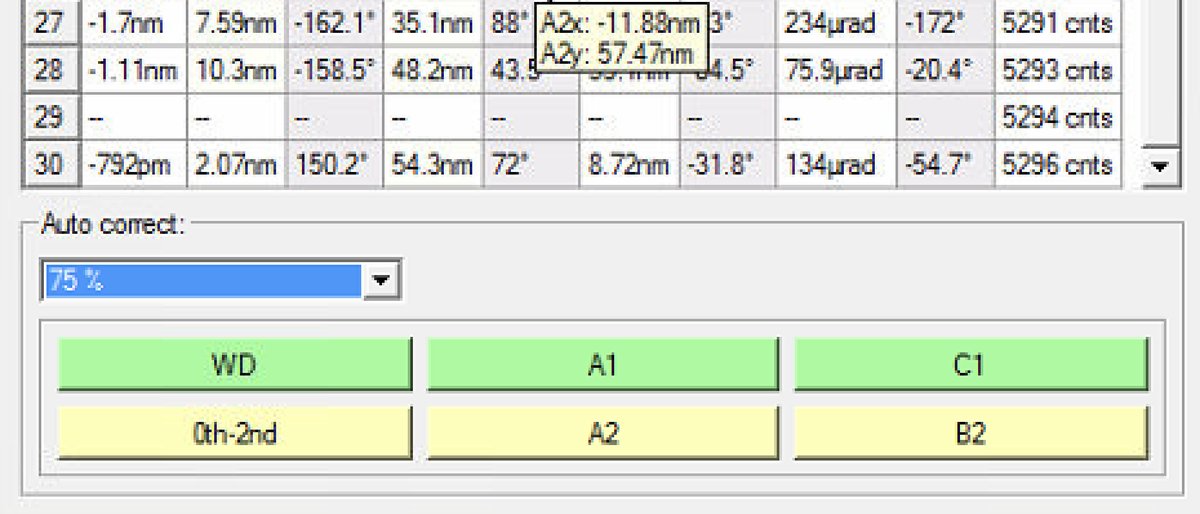
-
When to stop: C1A1 values are stable when they no longer decrease significantly between iterations. Target: C1 (defocus) < 1 nm and A1 (astigmatism) < 3 nm. Click
Stopwhen values are stable.
-
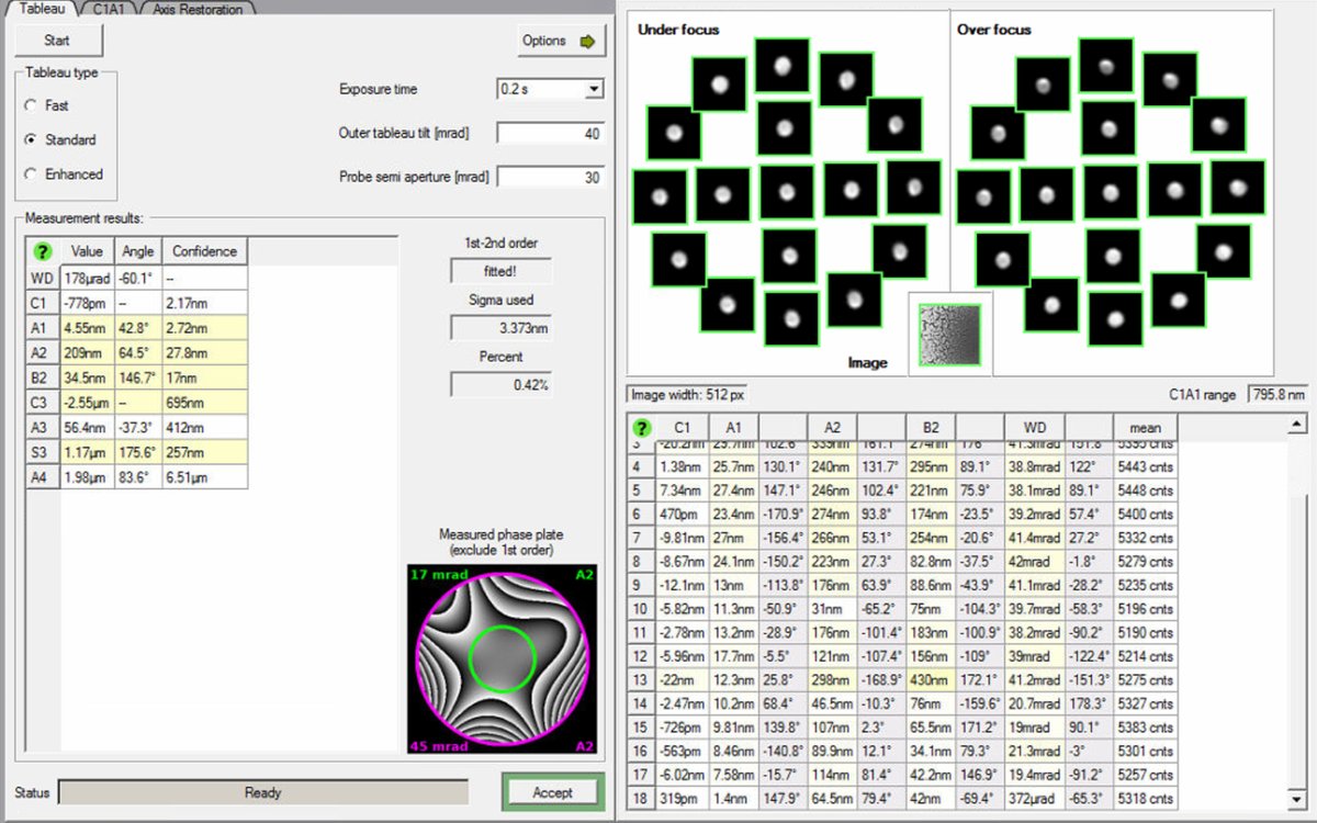
2.2 Tableau measurement
Tableau measures higher-order aberrations (A2, B2, C3, S3, A3) by acquiring ronchigram patterns at multiple beam tilt angles. The software analyzes how the ronchigram changes with tilt to extract the full aberration function. Tableau is more comprehensive than C1A1 and necessary for highest resolution.
-
Open Tableau tab
-
Switch to the
Tableautab in theProbe Correctorsoftware for full aberration measurement and correction. -
Select
Standardfor Tableau type. This acquires a sufficient number of tilt positions for accurate measurement without taking excessive time. -
Set the Outer tableau tilt to 40 mrad. Larger tilts probe higher-order aberrations but require more time.
-
Verify the Probe semi aperture is set to 30 mrad to match the beam settings.
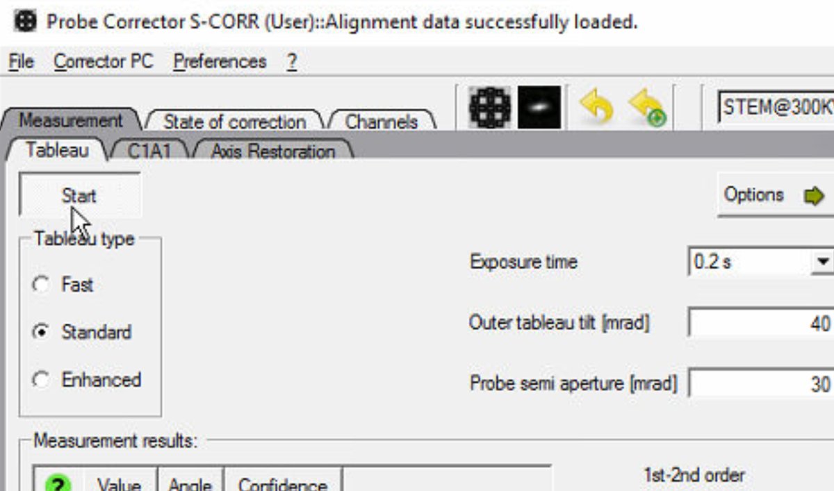
-
Click
Optionsand select theA5toggle. It measures up to 5th order aberrations.
-
-
Run Tableau measurement
-
Click
Startto begin the Tableau measurement. The software automatically tilts the beam to multiple angles and acquires ronchigram images at each position. -
Wait for measurement completion. The ronchigram shifts across the screen as the software captures patterns at different tilts and focus levels (under-focus and over-focus at each tilt). This movement is expected.
-
Do not modify the stage position during measurement. If the beam is unstable, stop and ask staff.
-
-
Accept measurement
- Click
Acceptafter measurement completes. This validates the data for corrections.
- Click
-
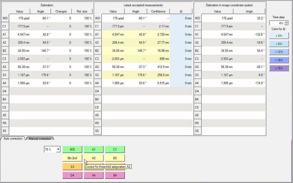
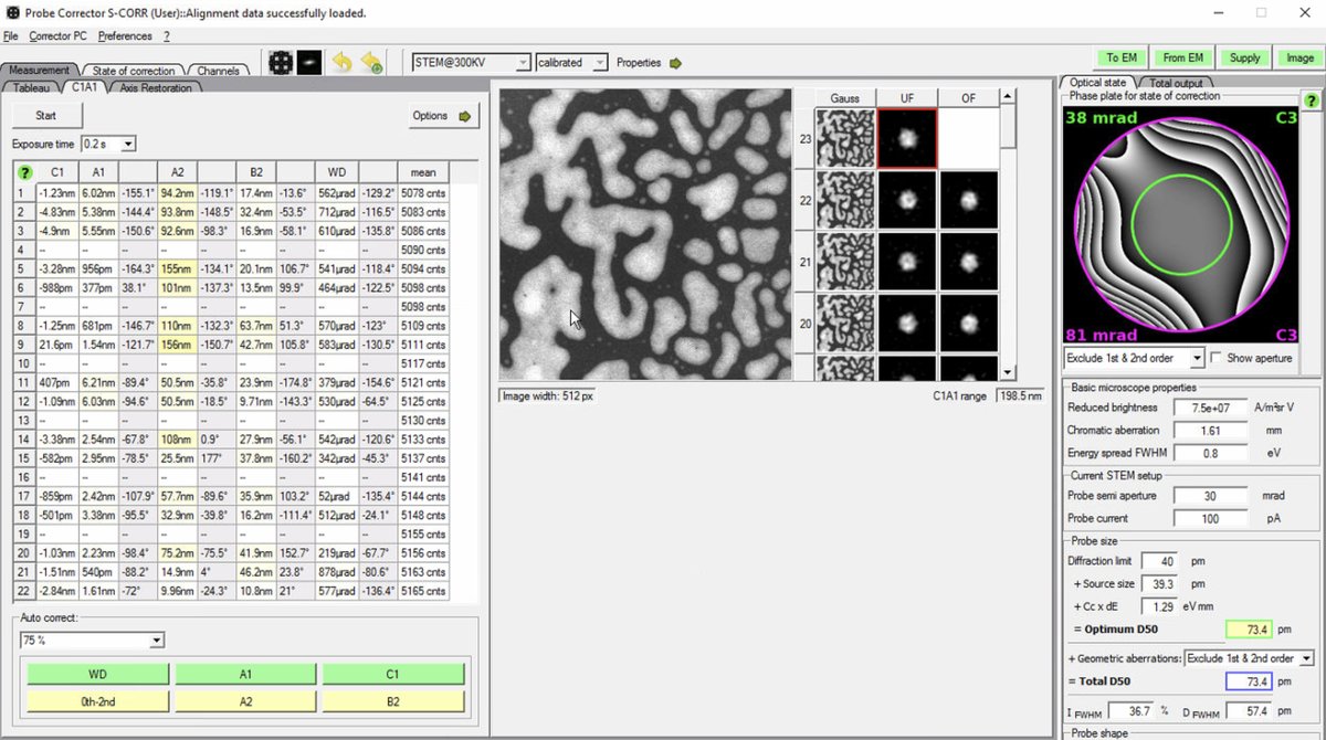
Review measurement results
-
Click the
State of correctiontab. This shows all measured aberration coefficients in three columns:- Estimation: Just measured values
- Latest accepted measurements: Previously applied corrections (yellow = outside limits)
- Estimation in image coordinate system: Values transformed to image coordinates
-
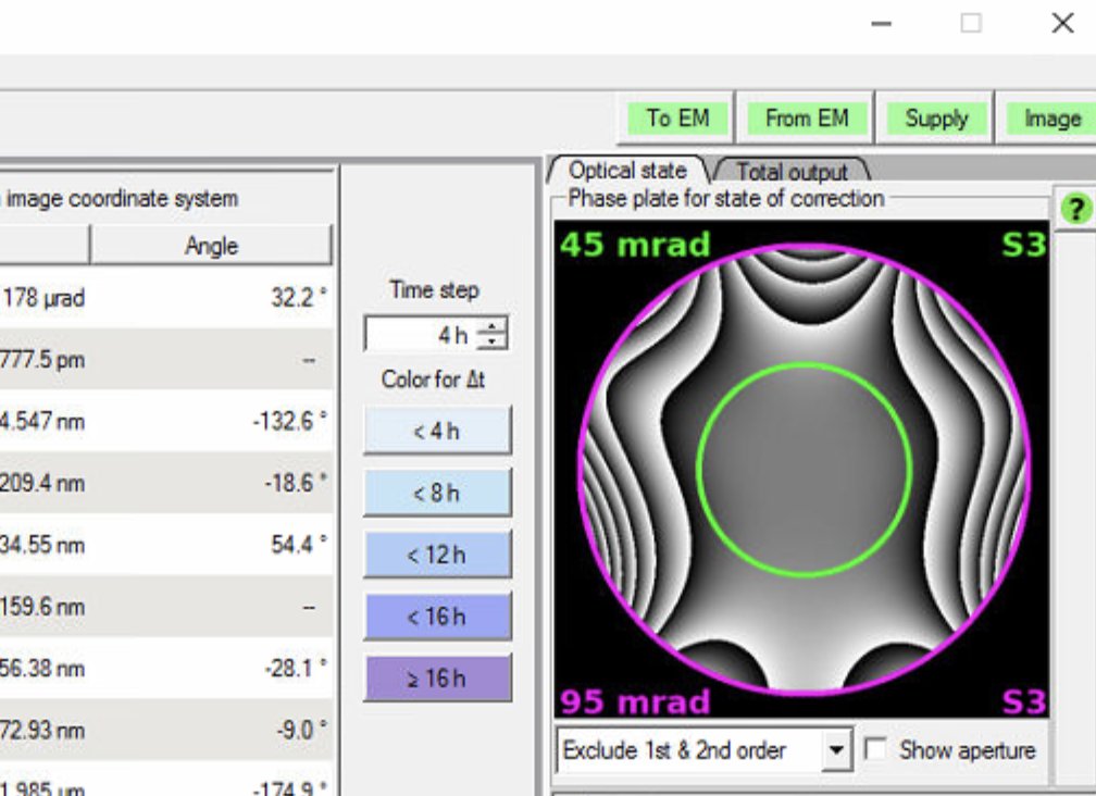
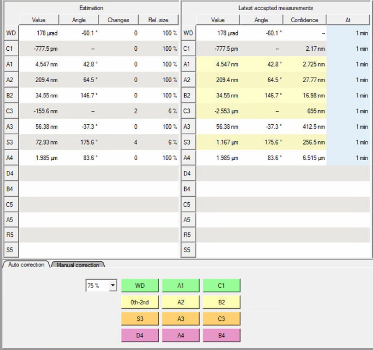
Check the phase plate visualization on the right. A well corrected probe has a flat, symmetric phase plate. Strong asymmetric patterns indicate uncorrected aberrations:
-
-
Apply corrections
-
Set Auto correct to 75% to prevent overcorrection. Yellow highlighted values in the “Latest accepted measurements” column indicate aberrations outside acceptable limits. Correct these first. In this example, S3 (1.167 μm) and C3 (-2.553 μm) are highlighted yellow:
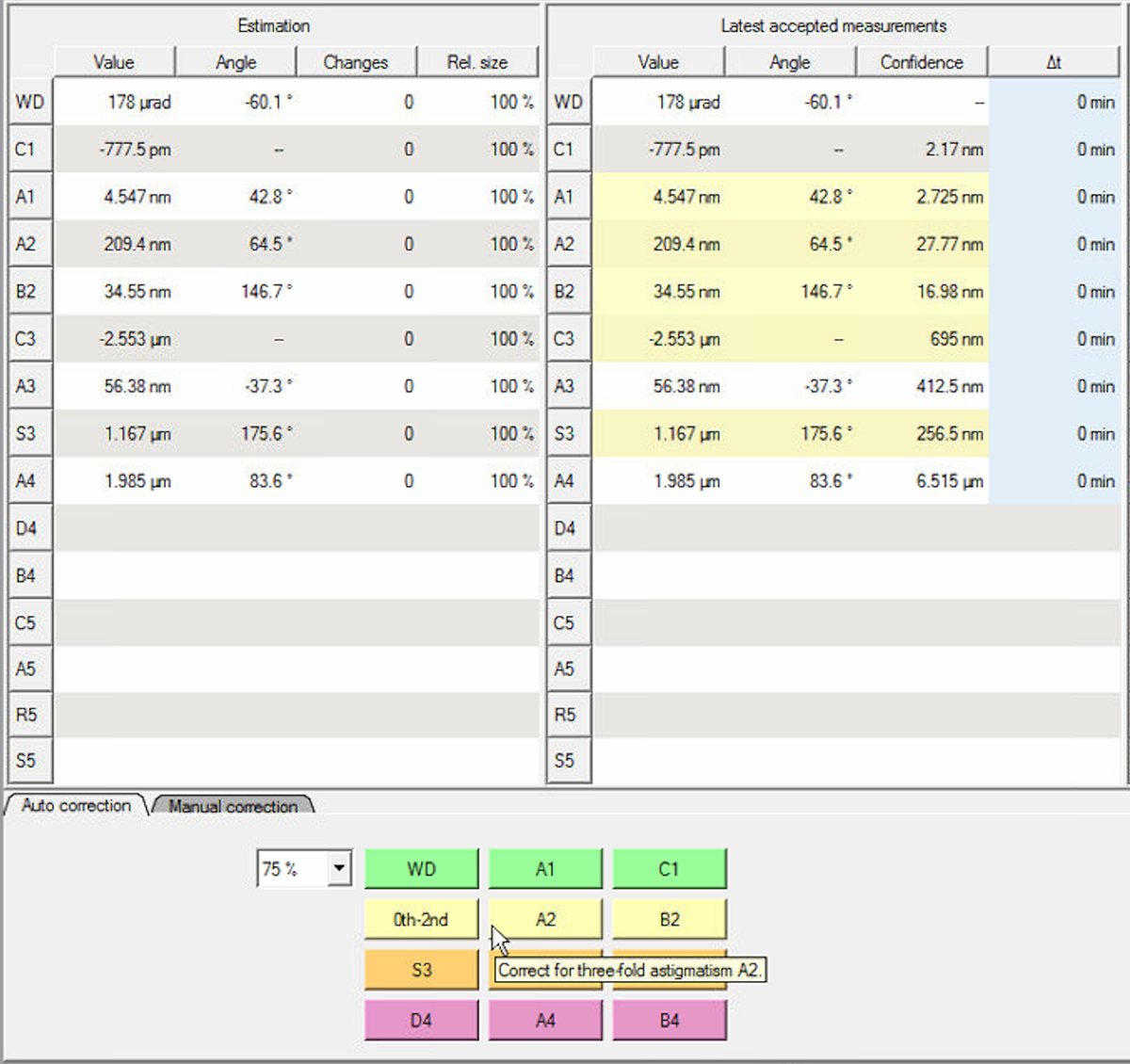
Note: either clicking
B4orD4can have a significant impact onC1andA1values.-
Click the aberration buttons at the bottom to apply corrections. The phase plate visualization shows the limiting aberration. Correct this one first. Click the button repeatedly until the value improves sufficiently, then move to the next limiting aberration.
-
The “Changes” column tracks how many corrections have been applied. After correcting S3 and C3, the values improve significantly:
- S3: 1.167 μm → 72.93 nm
- C3: -2.553 μm → -159.6 nm
-
-
Run full measurement
-
After applying corrections, run another complete Tableau measurement to verify the improvements.
-
Check the aberration surface and phase plate displays. A well-corrected probe shows:
- Flat aberration surface with green in the center (minimal phase variation across the aperture)
- Symmetric phase plates without strong directional features
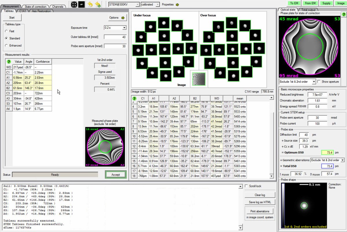
Target values (30 mrad semi-aperture):
Parameter Target C1 < 1 nm A1 < 3 nm A2 < 40 nm B2 < 25 nm C3 < 1.5 μm A3 < 1 μm S3 < 500 nm TODO: CONFIRM WITH ANDREW for IDEAL TOTAL D50
-
-
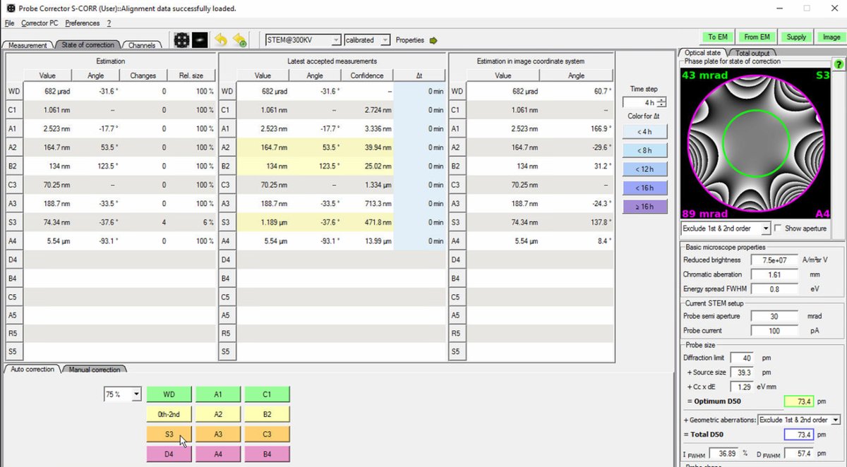
Verify with C1A1
- Return to the
C1A1tab in the Probe Corrector software. Tableau correction can sometimes introduce small first-order errors. - Click
Startto begin C1A1 measurement again. - Click
A1to correct any residual astigmatism introduced by Tableau. - Click
0th-2ndif defocus also needs adjustment. - Iterate between Tableau and C1A1 if necessary until all values are within specification.
- Return to the
-
Check resolution
-
The
State of correctionpanel displays resolution estimates on the right side: Total D50 and Optimum D50. D50 represents the probe diameter containing 50% of the beam intensity (smaller = better resolution).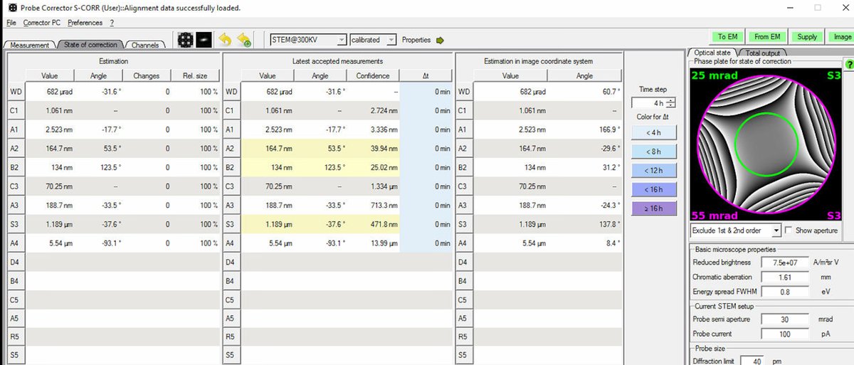
TODO: CONFIRM WITH ANDREW
-
Target: Total D50 of 70-75 pm for high-resolution STEM imaging. The Optimum D50 shows the theoretical best achievable with current aberrations. If these values match closely, corrections are complete.
-
If D50 values are significantly higher than target, continue iterating: run another Tableau measurement, apply corrections, then verify with C1A1. The image below shows C1A1 iterations after Tableau corrections:
-
-
Return to probe image mode
- Once correction is complete, press the
Diffractionbutton on the hand panel to switch back to probe image mode (STEM scanning). - The system is now ready for high-resolution image acquisition.
- Once correction is complete, press the
Part 3: Imaging
3.1 Acquire images
With aberration correction complete, the system is ready for high-resolution STEM image acquisition. The probe is optimized for atomic-resolution imaging.
-
Acquire HAADF image
-
In
Velox, clickSTEMto enter STEM mode, then clickHAADFto select the HAADF detector. -
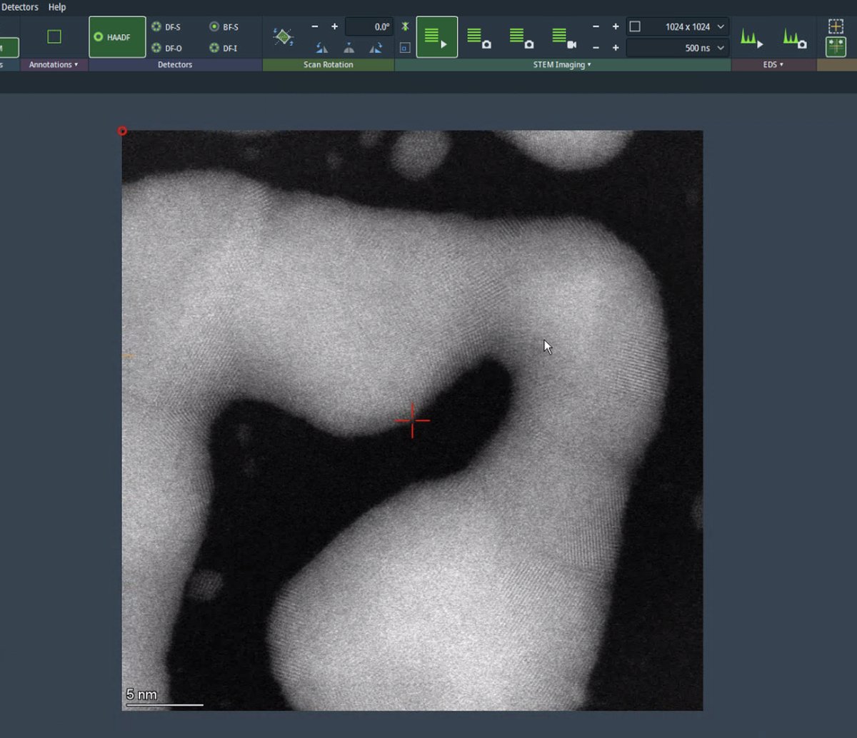
Click the play button to start live scanning. Image quality is noticeably improved compared to before correction. A well-corrected probe produces sharper, more detailed images.
-
For initial survey imaging, set resolution to 1024×1024 and dwell time to 500 ns. Fast scanning enables navigation while maintaining image quality.
-
-
Navigate to area of interest
-
Use the live scan to find the region of interest. Use the joystick or click on the image to move to different regions. With a well-corrected probe, atomic lattice fringes are visible in crystalline materials.
-
Adjust focus using the z-height controls if needed. Small focus changes can significantly affect atomic-resolution contrast.
-
-
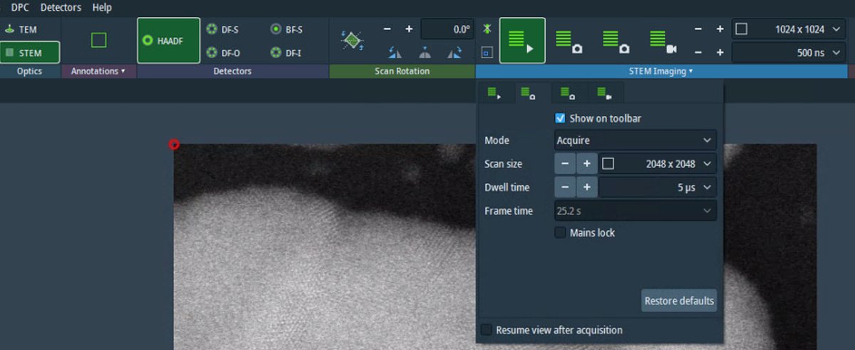
Capture high-resolution scan
-
Increase the resolution to 2048×2048 or higher. Check the Velox toolbar to verify resolution and dwell time settings before starting the acquisition.
-
Increase the dwell time to 5 µs for better signal-to-noise ratio. Longer dwell times collect more electrons per pixel, reducing noise but increasing total scan time and potential for drift artifacts. After acquisition completes, the beam is blanked automatically to prevent sample damage.
-
3.2 Fine-tuning with Sherpa
Sherpa provides rapid aberration correction that is faster than full Tableau measurement. Use Sherpa for quick refinements after the main alignment, or when aberrations drift during extended imaging sessions.
-
Prepare for Sherpa
-
Before running Sherpa, verify the ronchigram is centered. Press the
Diffractionbutton on the hand panel to switch to diffraction mode (view the ronchigram). -
In
TEMUI, go toDirect Alignmentsand selectDiffraction Shift and Focus alignment: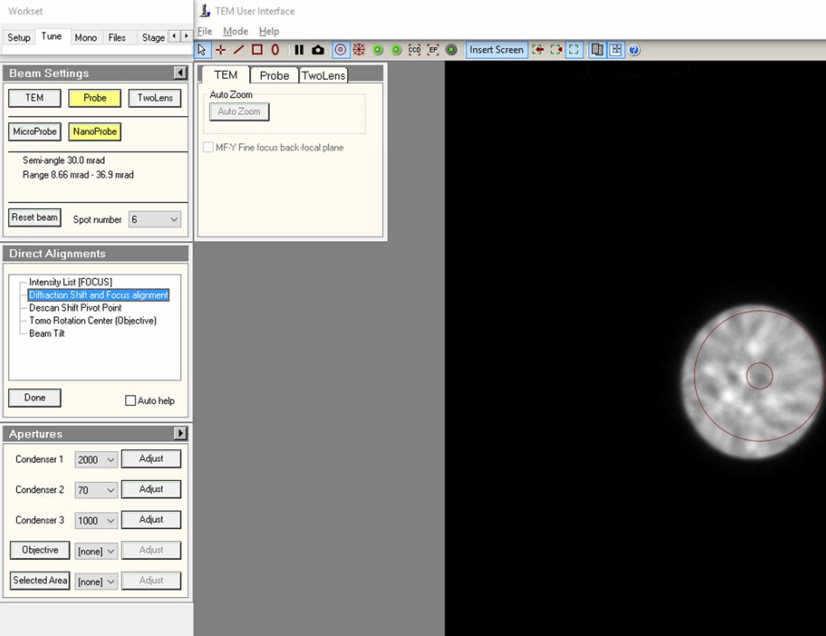
-
Use the
mulXYknobs to center the ronchigram on the display. A centered ronchigram ensures Sherpa measurements are accurate.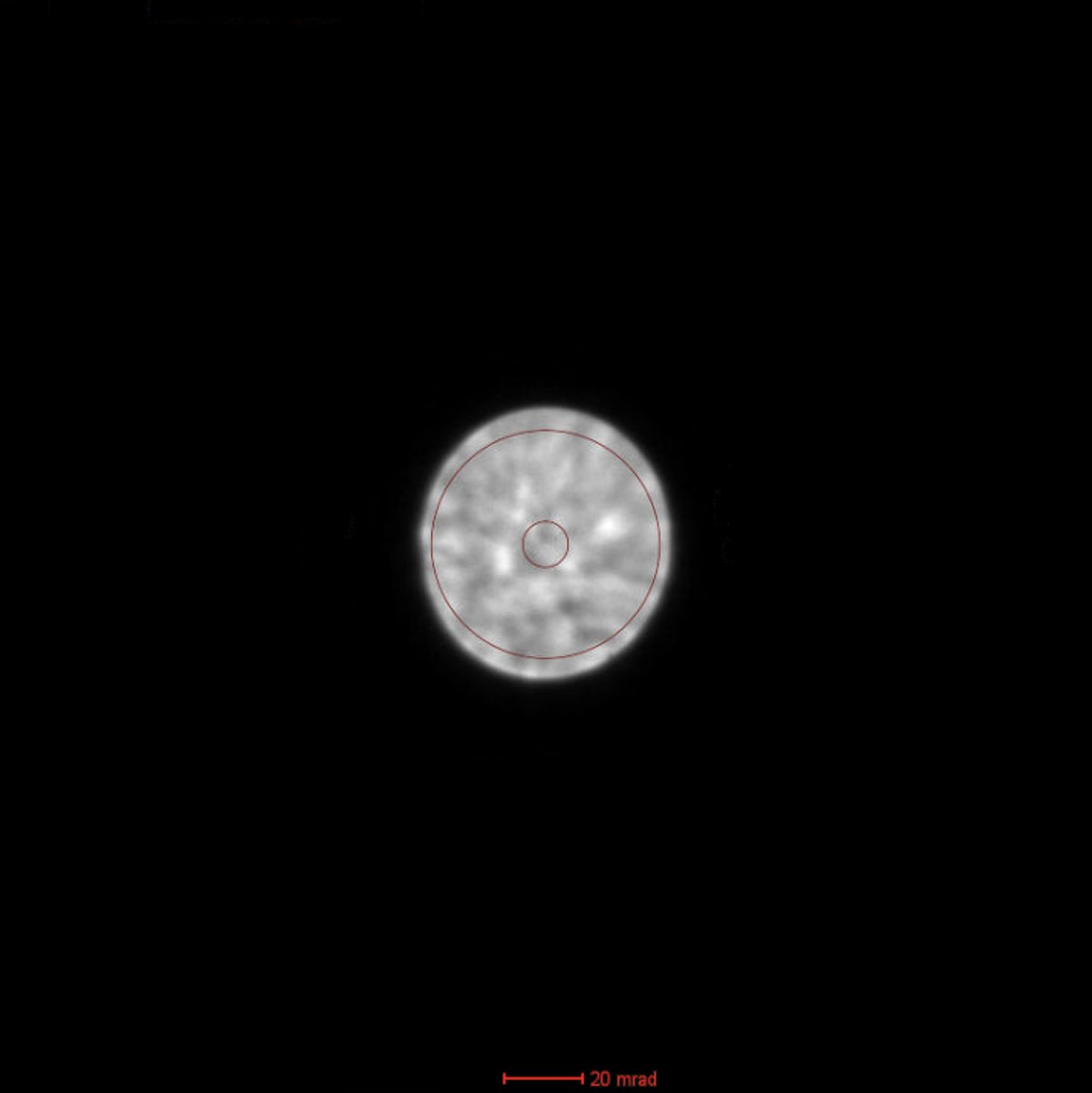
-
-
Adjust C2 aperture (optional)
-
To change C2 aperture size (for example, switching to 50 µm for different probe conditions), locate the
Aperturespanel and change Condenser 2 from 70 to 50 (or the desired size).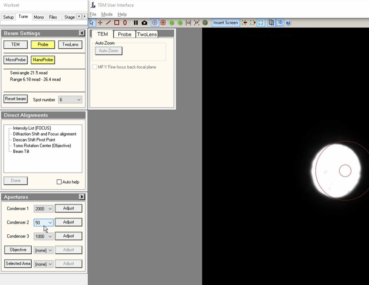
-
Click
Adjustto center the new aperture. The beam remains centered when changing aperture sizes. If not centered, use the adjustment controls to re-center.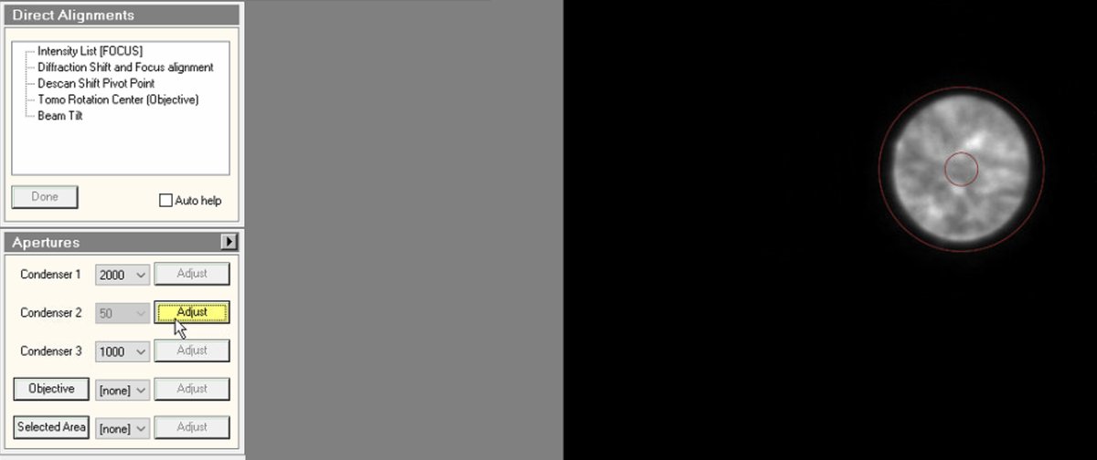
-
-
Open Sherpa
-
Open the
Sherpasoftware. Sherpa displays the HAADF image with a crosshair marker indicating the measurement region.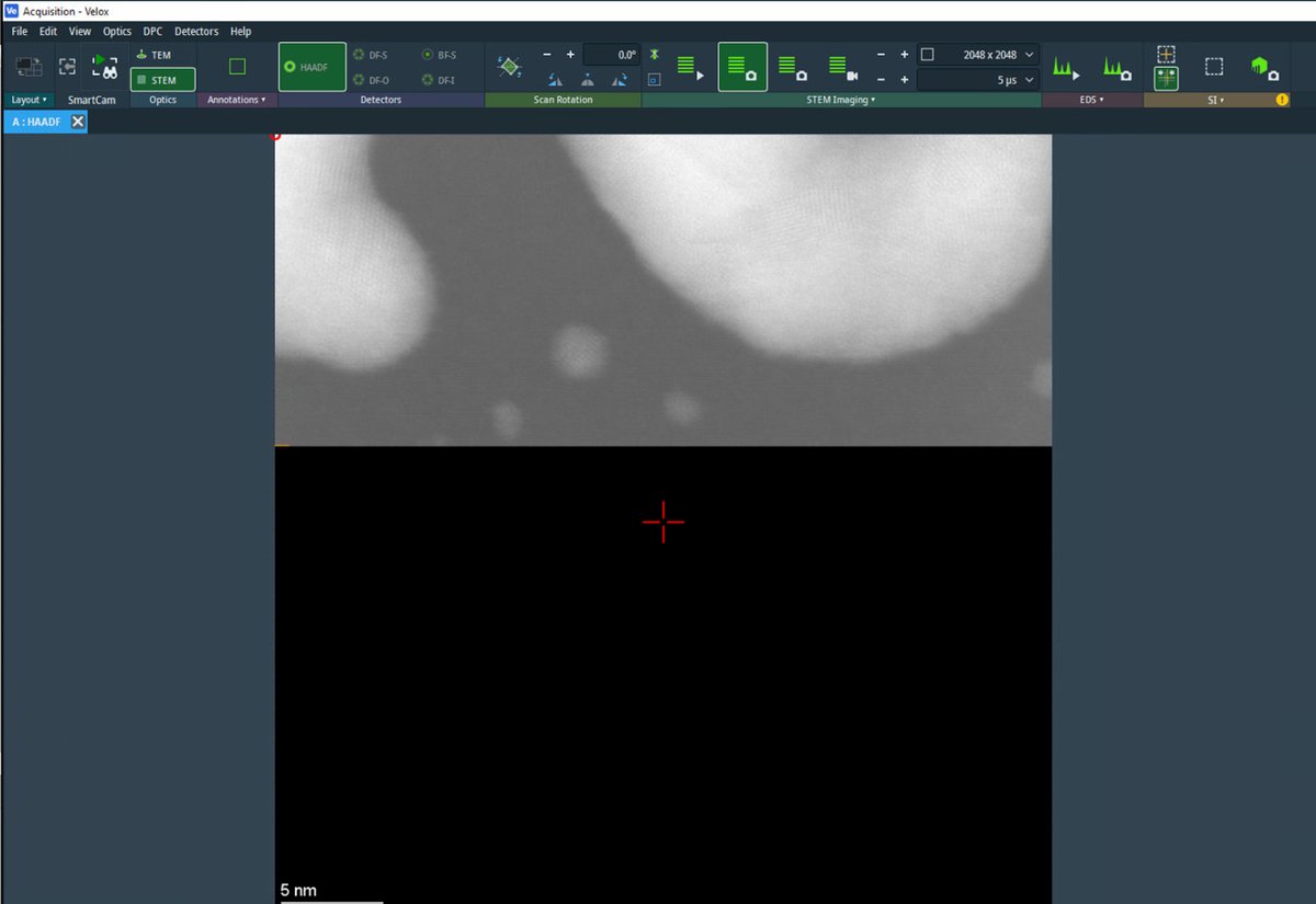
-
Click
C1/A1to run first-order correction (defocus and 2-fold astigmatism).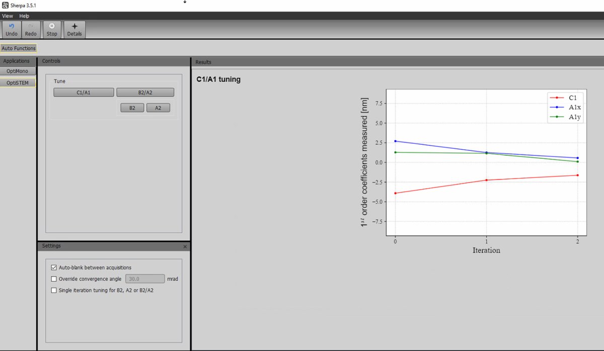
-
-
Run B2/A2 tuning
-
After C1/A1 completes, click the
B2/A2button to correct second-order aberrations (axial coma B2 and 3-fold astigmatism A2). -
Wait for the tuning to complete. Sherpa acquires images and determines optimal corrections.
-
Run multiple iterations if the first pass does not achieve optimal results.
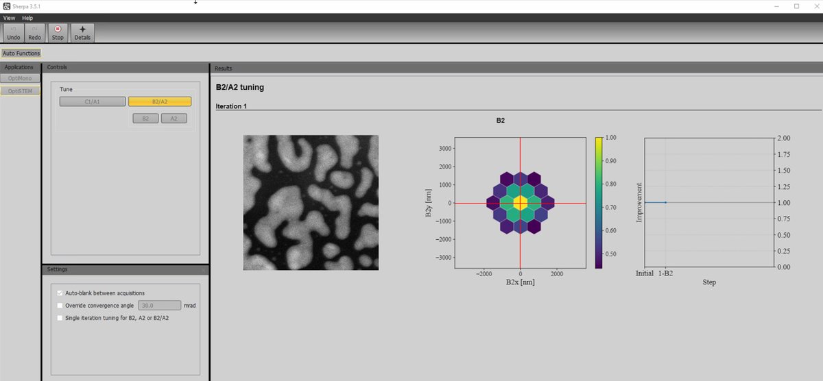
-
-
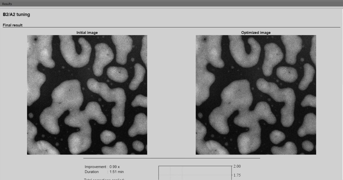
Review results
-
Sherpa displays the initial image alongside the optimized image for comparison. The corrected image shows improved sharpness and resolution.
-
3.3 Load your own sample
After completing probe correction on the standard sample, follow the below steps unload the current sample standard and load your own. For holder-specific instructions (single-tilt, double-tilt, tomography), see Sample Loading.
-
Remove the standard sample
-
Put on gloves before handling any holders or samples.
-
Blank the beam and verify the screen is inserted. The screen protects the detectors and cameras below from the beam.
-
Close the column valves by pressing
Column Valves Closed.If a “VCP” error occurs, follow the instructions on the Spectra NEMO page.
-
Reset the holder by clicking
reseton theStagemenu.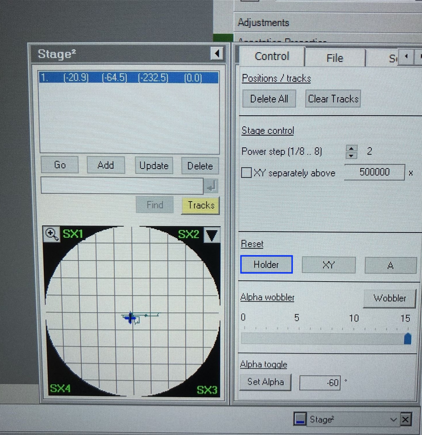
-
Confirm the stage x, y, z values are returning to zero after you reset the holder stage.
-
Pull the holder straight out to the first resistance point. Do not force beyond this point. Turn clockwise, then pull the rest of the holder out continuously.
-
-
Load your sample and insert the holder
IMPORTANT: Do not remove the standard sample from the single-tilt holder. Use a separate holder to load your sample.
-
For holder-specific loading instructions, see Sample Loading.
-
Align the holder with the blue line on the goniometer.
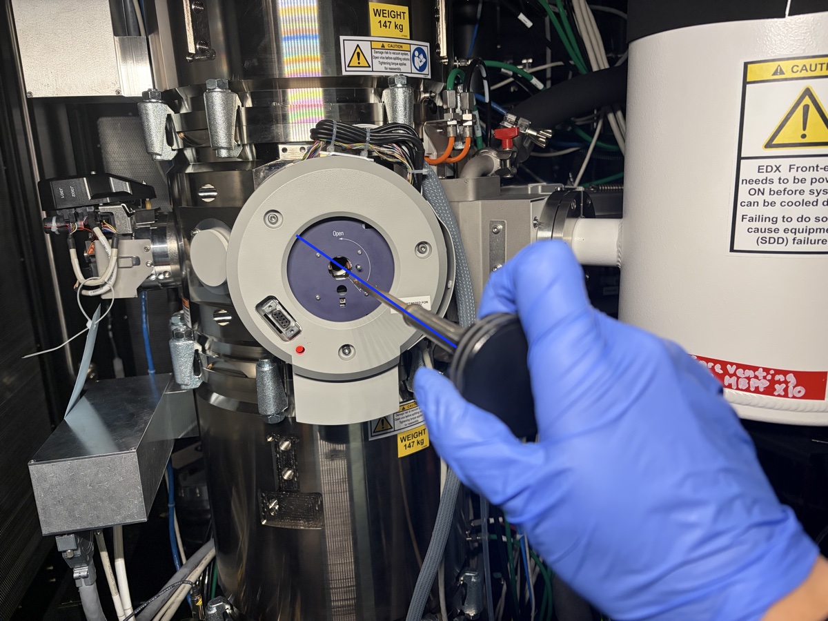
-
Push the holder in until you feel resistance. Do not push all the way in.
-
The turbo pump starts automatically. Wait ~2 minutes for pressure to stabilize. You can monitor the time in
TEMUIor on the screen attached to the Spectra instrument.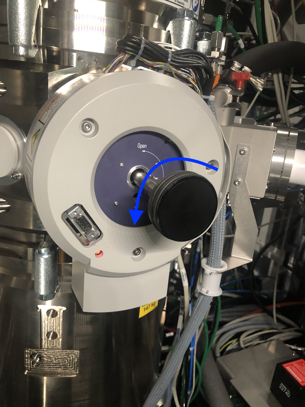
Why wait? The holder insertion opens a small chamber to atmosphere. The turbo pump must evacuate this air before you can insert the holder into the main column. Rushing this step would introduce air into the ultra-high vacuum column, potentially damaging the electron gun and contaminating the system.
-
Wait until the PPII gauge drops into the high 10⁻⁶ mbar to low 10⁻⁷ mbar range before continuing. PPII reads the load lock / projection chamber pressure; the holder insertion path is only safe to advance once PPII has reached this range.
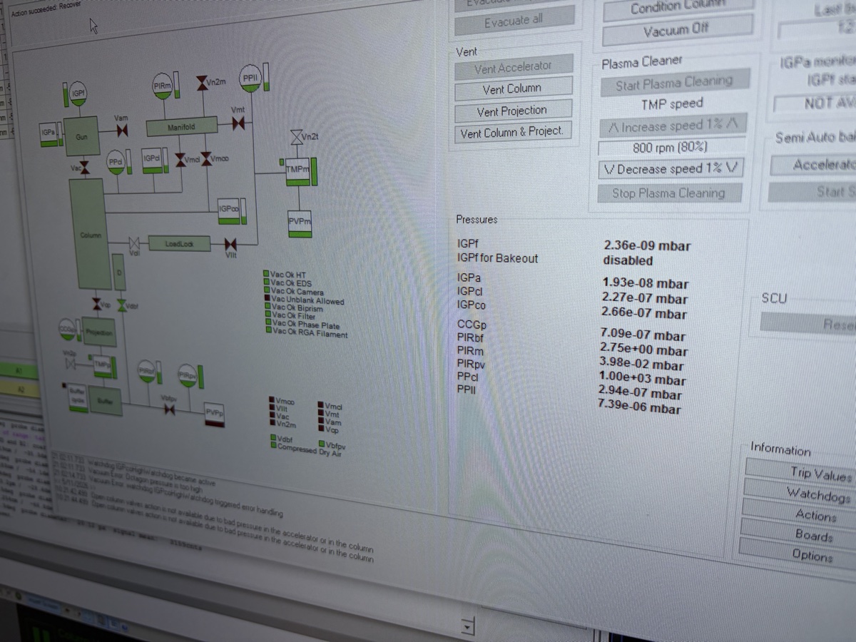
NOTE: In the example above PPII reads 7.39 × 10⁻⁶ mbar (high 10⁻⁶ range), which is right at the threshold. Wait until it drops further (low 10⁻⁶ or into 10⁻⁷) for a more conservative margin before the next step.
-
Turn the holder counter-clockwise until you feel gently stuck, then guide the holder to push in. The holder should move in smoothly.
-
In
TEMUI, turn off the turbo pump. Confirm the holder type when prompted.
-
Re-do eucentric height
- Open column valves and re-do eucentric height for your new sample (1.3). Each sample sits at a different physical height in the holder. Find the ronchigram “blow-up” point again so the sample stays centered when tilted and the probe is properly focused.
- Run a quick C1A1 or Sherpa to verify probe correction still holds after the sample change. For beam-sensitive or low-contrast samples where Sherpa cannot be used, see Manual Aberration Correction (Advanced).
Part 4: End session
4.1 Reload the standard sample
-
Reload the standard sample
-
Put on gloves before handling any holders or samples.
-
Blank the beam and verify the screen is inserted.
-
In
TEMUI, clickColumn Valves Closed. -
Click
Reset Holderunder theStagemenu. Visually verify that the X, Y, and Z stage coordinates are reset after the button is pressed.
-
Pull the holder with your sample straight out to the first resistance point. Do not force beyond this point. Turn clockwise, then pull the rest of the holder out continuously.
-
Set aside your holder and pick up the single-tilt holder with the standard sample.
-
Push the single-tilt holder with the standard sample in until you feel resistance. Do not push all the way in.
-
The turbo pump starts automatically. Wait ~2 minutes for pressure to stabilize.
-
Turn the holder counter-clockwise until you feel gently stuck, then guide the holder to push in.
-
In
TEMUI, turn off the turbo pump. ConfirmSingle tilton TEMUI.
-
4.2 Checklist before leaving the Spectra room
- Beam is blanked.
-
Reset Holderhas been pressed and X, Y, Z stage coordinates are verified reset. - Stage is returned to 0° tilt (alpha and beta).
- Arina detector is retracted, verified on the left hand panel.
- Arina detector is turned off, verified on the local Firefox URL.
-
INT SCANphysical button is in pressed state. - Screen is inserted.
- Column valve is closed.
- Turbo pump is turned off.
- Standard sample is loaded.
- All holders are capped and stored in the holder box.
- The sample loading area is tidy.
- Spectra usage is terminated on NEMO.
- Internet accounts (Google, Outlook, etc.) are signed off.
- Fill out the logbook if anything unusual happened during the session.
Troubleshooting
Common problems encountered during STEM sessions.
| Problem | Cause | Solution |
|---|---|---|
| Image drifts when tilting | Eucentric height not set | Re-do eucentric height after loading a new sample |
| C1A1 measurements unstable or fail | Velox is still scanning | Stop live scanning in Velox before running C1A1, then verify the beam is unblanked |
| Aberration values oscillate instead of converging | Overcorrection percentage too high | Start with 100% Auto correct, reduce to 75% as values approach target |
| C1A1 or Tableau shows no signal | Beam is blanked | Click Beam Blank button to unblank before running aberration measurements |
| Good Tableau values but poor image resolution | Missing C1A1 verification step | After Tableau, always run C1A1 again to fine-tune defocus and astigmatism |
| Beam disappears from view | Random adjustments displaced the beam | Go to lower magnification until beam is visible, use joystick to move sample to center, then go to Diffraction Shift and use mulXY to center the beam |
| Lost beam or need to redo alignment | Column misalignment after extended session | Redo eucentric height (1.3) and monochromator tune (1.6). If you cannot find the sample, switch to TEM mode for easier navigation (TEM Spectra) |
FAQ
Beam blanking
When the beam is blanked, the electron beam is deflected away from the sample so no electrons hit it. This prevents unnecessary radiation damage to the sample when not actively imaging. The beam is automatically blanked when scanning stops or after taking a picture. Manual blank/unblank is available via the Beam Blank button on the hand panel or in the software.
Monochromator focus adjustment
The monochromator filters the energy spread of the electron beam by passing it through a narrow slit. Setting Focus = 0 places the beam crossover exactly at the monochromator slit plane. This position maximizes electron throughput while maintaining energy filtering. If the focus is offset from zero, the beam crossover occurs before or after the slit, reducing beam current and degrading energy resolution.
Appendix
Aberration notation
Different notations exist for aberrations in the literature. The table below shows the Krivanek notation (used in Probe Corrector software), the alternative notation (used in this guide), and descriptions.
| Krivanek | Alt | Description | Krivanek | Alt | Description |
|---|---|---|---|---|---|
| \(C_{10}\) | \(C_1\) | Defocus | \(C_{41}\) | \(B_4\) | 4th order coma |
| \(C_{12}\) | \(A_1\) | 2-fold astigmatism | \(C_{43}\) | \(D_4\) | 3-lobe aberration |
| \(C_{21}\) | \(B_2\) | Axial coma | \(C_{45}\) | \(A_4\) | 5-fold astigmatism |
| \(C_{23}\) | \(A_2\) | 3-fold astigmatism | \(C_{50}\) | \(C_5\) | 5th order spherical |
| \(C_{30}\) | \(C_3\)/\(C_s\) | Spherical | \(C_{52}\) | \(S_5\) | 5th order star |
| \(C_{32}\) | \(S_3\) | Star aberration | \(C_{54}\) | \(R_5\) | Rosette |
| \(C_{34}\) | \(A_3\) | 4-fold astigmatism | \(C_{56}\) | \(A_5\) | 6-fold astigmatism |
Changelog
- May 6, 2026 - Promote End session to Part 4 and add it to the overview table
- Mar 1, 2026 - Add pre-session checklist, sample loading section with glove requirement, end session with explicit reload steps, fix image paths
- Feb 28, 2026 - Add prerequisite link to TEM Alignment guide; add lost-beam troubleshooting
- Jan 31, 2026 - Initial draft: instructions by Sangjoon Bob Lee, screenshots by Andrew Barnum during Spectra 300 hands-on training