From acquisition to images

Load Gold → inspect mean diffraction, BF, ADF and DPC → reconstruct SSB phase. Everything needed for a first reconstruction is on this page, using one acquisition throughout. No QEM conversion is required first.

Follow the installation guide and install huggingface_hub for the download. QuantEM selects the available GPU automatically. For probe images, fitted coefficients, search trials, upsampling, and saved results, use the advanced Gold tutorial.

Get the Gold data

The public Gold acquisition contains a 512 × 512 scan and 48 × 48 detector. Only the detector was binned by four before upload. The download is about 1.2 GB, is MIT licensed, and stays in data/ for reuse.

from pathlib import Path
import json

from huggingface_hub import snapshot_download
from quantem.gpu import io, detector, dpc, SSB
from quantem.core.visualization import show_2d

snapshot_download(
    "bobleesj/quantem-data", repo_type="dataset",
    revision="00179851c0015612bfb6e6438e02387f5ffff0ae",
    allow_patterns="4dstem/gold_512_npy_bin4/*", local_dir="data", token=False,
)
folder = Path("data/4dstem/gold_512_npy_bin4")
metadata = json.loads((folder / "meta.json").read_text())

The metadata supplies 300 kV, a 30 mrad convergence semiangle, and 1.84 mrad per detector pixel. Its 0.5 Å scan spacing was inferred from a sibling acquisition, not independently calibrated for this file. Scale bars below retain that qualification.

Load and view the mean diffraction pattern

data = io.load(folder / "data.npy")
mean_dp = detector.mean(data)
show_2d(
    mean_dp, title="Gold mean diffraction pattern", norm="log_auto",
    cmap="inferno", axsize=(3.5, 3.5),
    scalebar={"sampling": metadata["sampling"][2], "units": "mrad"},
)

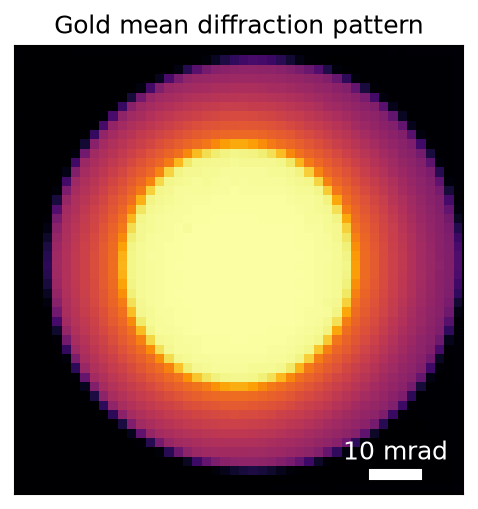
This averages all scan positions, leaving the 48 × 48 detector image. Inspect the bright central disk and surrounding scattering before reconstructing. Logarithmic display contrast makes weak scattering visible. The scale is angular: detector pixels describe scattering directions, not sample positions.

View bright field, dark field, and DPC

bf = detector.bf(data)
adf = detector.adf(data)
dpc_result = dpc.run(data)
show_2d(
    [bf, adf, dpc_result.phase], title=["BF", "Annular dark field", "Integrated DPC"],
    norm=["power_sqrt", "power_sqrt", "minmax"], cmap="inferno", axsize=(3, 3),
    scalebar={"sampling": metadata["sampling"][0], "units": "Å"},
)
dpc_result.rotation_deg, dpc_result.use_transpose  # degrees; detector-axis swap flag

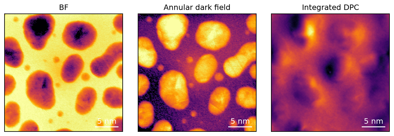
All three panels show the same 512 × 512 scan. BF integrates the central disk; ADF is annular dark field, integrating the surrounding ring. The detector finds the disk automatically. Integrated DPC comes from the measured center-of-mass shifts. Its displayed contrast is not calibrated in radians. Each panel uses independent contrast: square-root for BF/ADF and linear for DPC.

DPC estimates the scan–detector rotation. This Gold acquisition reports use_transpose=False, so pass the angle directly to SSB. For other data, check that value first: a detector-axis swap must be resolved before reusing the angle alone. SSB does not run DPC automatically.

Reconstruct SSB phase

Reuse the same acquisition and the DPC rotation above.

ssb = SSB(
    data,
    voltage_kV=metadata["voltage_kV"],  # kV
    semiangle_mrad=metadata["probe_semiangle_mrad"],  # mrad
    scan_sampling_A=metadata["sampling"][0],  # Å per scan pixel
    det_sampling=metadata["sampling"][2],  # mrad per detector pixel
    rotation_angle_deg=dpc_result.rotation_deg,  # degrees
)
aberrations = ssb.find_aberrations()
result = ssb.reconstruct(aberrations, upsample=1)
show_2d(
    result.phase, title="Gold SSB phase (rad)", cmap="inferno", cbar=True,
    scalebar={"sampling": result.scan_sampling_A, "units": "Å"},
)

SSB finds the bright-field disk automatically. find_aberrations() fits defocus and twofold astigmatism on the native grid; reconstruct() uses those parameters without repeating the search. Voltage, sampling, and convergence angle stay fixed. Specimen tilt and model depth spread are zero in this example.

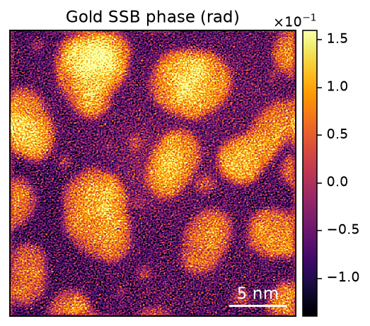
This is the 512 × 512 native reconstruction: 0.5 Å per output pixel and a 25.6 nm square field using the supplied calibration. Experimental Gold has no known specimen potential here; the image does not establish quantitative phase accuracy in the thicker particles. Use 1× for this example: the current 4× implementation produces stripes. The advanced comparison shows the same region at both factors.

Data axes are (scan_rows, scan_cols, detector_rows, detector_cols). To view one measured pattern, use show_2d(data[256, 256], norm="power_sqrt", cmap="inferno"). The advanced disk-geometry example draws the fitted center and radius on the mean pattern. I/O covers detector crops and 5D acquisition selection; Detector and DPC covers manual radii and physical-angle units.

Finish, or inspect further

Keep the session open for the advanced tutorial:

Inspect or save	Example
Fitted coefficients and search candidates	Read the aberration search
Phase beside the model probe	Build the probe image
Native versus 4× phase	Compare the same field and particle
Measurements and calibration in one file	Save as QEM

When finished, close the session before its acquisition:

ssb.close()
data.close()