Gold: data loading, detectors and SSB

Use the public Gold acquisition to load diffraction patterns, inspect detector images, save and reopen QEM, and reconstruct SSB phase. The download is pinned to a dataset revision. Use your own microscope calibration when adapting this workflow to another acquisition.

The later cells compare native and 4× phase sampling and show the calculated real-space and Fourier-space model probes.

Download the data

The two files stay in data/. The fixed revision keeps repeat downloads on the same dataset.

from pathlib import Path
import json

from huggingface_hub import snapshot_download
from quantem.gpu import io, detector
from quantem.core.visualization import show_2d

revision = "00179851c0015612bfb6e6438e02387f5ffff0ae"
download = snapshot_download(
    "bobleesj/quantem-data", repo_type="dataset", revision=revision,
    allow_patterns="4dstem/gold_512_npy_bin4/*", local_dir="data", token=False,
)
folder = Path("data/4dstem/gold_512_npy_bin4")

Load and look

io.load opens the measurements on the GPU. NumPy files do not carry calibration, so we read the accompanying meta.json separately.

data = io.load(folder / "data.npy")
metadata = json.loads((folder / "meta.json").read_text())
data.shape, data.dtype

Loaded uint16 measurements as uint16 ANS on cuda; no binning or cropping.

((512, 512, 48, 48), dtype('uint16'))

Mean diffraction pattern and disk geometry

Average over the scan positions, then estimate the bright-field disk’s center and radius. Both are in detector pixels; the center uses (row, column) order. This finds the disk geometry, not the probe phase or defocus.

mean_dp = detector.mean(data)
center, radius = detector.fit_probe(mean_dp)  # (row, column) and radius, detector pixels

from matplotlib.patches import Circle

fig, ax = show_2d(
    mean_dp, title="Mean diffraction pattern and fitted disk",
    norm="log_auto", cmap="inferno", axsize=(3.5, 3.5),
    scalebar={"sampling": metadata["sampling"][2], "units": "mrad"},
)
row, column = center
ax.add_patch(Circle((column, row), radius, fill=False, color="cyan"))
ax.plot(column, row, "+", color="cyan");

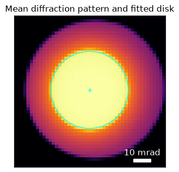
The cyan cross marks the center; the circle marks the fitted radius. Matplotlib takes (column, row) when drawing, so only the plotting call swaps that order.

BF and ADF images

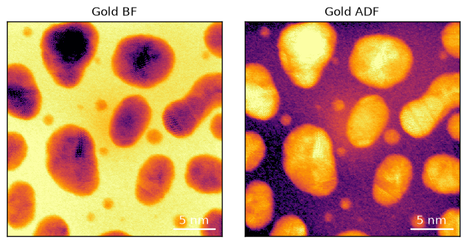
The first detector call finds the bright-field disk. BF integrates inside it; ADF integrates the default surrounding annulus. Each image has its own display contrast.

The scale bars use the supplied 0.5 Å per scan pixel. That spacing was inferred from a sibling acquisition, not calibrated for this file. We retain that qualification in the saved metadata.

bf = detector.bf(data)
adf = detector.adf(data)
show_2d(
    [bf, adf], title=["Gold BF", "Gold ADF"],
    norm="power_sqrt", cmap="inferno", axsize=(3.5, 3.5),
    scalebar={"sampling": metadata["sampling"][0], "units": "Å"},
);

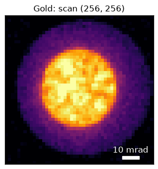
Select a diffraction pattern by scan (row, column). Its scale bar uses the detector spacing from the same metadata file.

pattern = data[256, 256]
show_2d(
    pattern, title="Gold: scan (256, 256)", norm="power_sqrt", cmap="inferno",
    axsize=(3.5, 3.5),
    scalebar={"sampling": metadata["sampling"][2], "units": "mrad"},
);

Save the acquisition

Save the measurements, map the supplied calibration to QEM fields, and keep the complete source JSON. No calibration values are guessed here. results/gold.qem stays on disk after the notebook finishes. If it already exists, choose a new filename before rerunning this cell.

Path("results").mkdir(exist_ok=True)
saved_file = "results/gold.qem"
export = io.save(saved_file, data, metadata={
    **data.metadata,
    "scan_sampling_A": metadata["sampling"][:2],
    "detector_sampling": metadata["sampling"][2:],
    "detector_sampling_unit": "mrad",
    "voltage_kV": metadata["voltage_kV"],
    "semiangle_mrad": metadata["probe_semiangle_mrad"],
    "source_metadata": metadata,
})
data.close()

Reopen and compare

The original acquisition is now closed. Open the QEM file and read the same pattern. The two panels use the same contrast limits.

saved = io.load(saved_file)
reopened_pattern = saved[256, 256]
show_2d(
    [pattern, reopened_pattern], title=["Before saving", "Reopened QEM"],
    norm="power_sqrt", cmap="inferno", axsize=(3.5, 3.5),
    vmin=0, vmax=float(pattern.float().max()),
    scalebar={"sampling": saved.sampling[2], "units": saved.units[2]},
);

Restored exact CUDA ANS (512, 512, 48, 48) in 0.438 s.

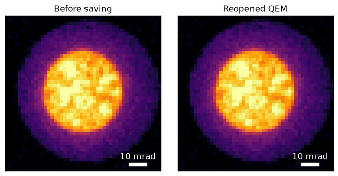
Check the selected pattern and BF image numerically. Looking identical in a plot is not enough.

saved  # the acquisition reports its shape, sampling and storage

Dataset4dstemGPU(shape=(512, 512, 48, 48), dtype=uint16, representation='encoded')

DPC and scan rotation

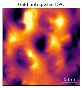
Use the reopened QEM acquisition to calculate the center of mass and integrated DPC image. DPC also estimates the scan–detector rotation. Here use_transpose is False, so we can pass the angle directly to SSB. For a different acquisition with True, resolve the detector-axis swap first; passing the angle alone does not apply that swap.

from quantem.gpu import dpc, SSB

dpc_result = dpc.run(saved)
show_2d(
    dpc_result.phase, title="Gold: integrated DPC",
    cmap="inferno", axsize=(3.5, 3.5),
    scalebar={"sampling": saved.sampling[0], "units": "Å"},
);

Find aberrations and reconstruct SSB

Use the recorded voltage, convergence angle and pixel spacings, together with the disk geometry and DPC rotation above. The scan spacing retains the calibration qualification stated earlier.

find_aberrations() always searches at native (1×) sampling; it has no upsample argument. It runs the default 200-trial search followed by Nelder–Mead refinement. It also checks the 180° rotation ambiguity using phase polarity. This is a heuristic, not an independent calibration measurement. reconstruct() applies the resulting parameters without another search.

This run fits defocus and twofold astigmatism. Specimen tilt and depth spread are held at zero. For the joint tilt/depth model, see the SSB API.

After the search, aberrations.report() displays the fitted values. Read defocus with aberrations["C10"] (nm). While the session remains open, ssb.show_trials(best=5), ssb.show_trials(last=5) or ssb.show_trials(first=5) lets you inspect candidate reconstructions. The SSB API documents trial replay and saved-result loading.

ssb = SSB(
    saved,
    voltage_kV=metadata["voltage_kV"],  # kV
    semiangle_mrad=metadata["probe_semiangle_mrad"],  # mrad
    scan_sampling_A=saved.sampling[0],  # Å per scan pixel
    det_sampling=saved.sampling[2],  # mrad per detector pixel
    bf_center=center, bf_radius=radius,  # detector pixels; center (row, column)
    rotation_angle_deg=dpc_result.rotation_deg,  # degrees
    source_path=saved_file,
)
aberrations = ssb.find_aberrations(save_to="results/gold-aberrations", verbose=False)
aberrations.report()

	C10 (nm)	C12 (nm)	phi12 (deg)	Suggested rotation (deg)	SSB-selected rotation (deg)
model
standard SSB	-22.398	-3.321	50.135	177.989	357.989

result = ssb.reconstruct(aberrations, upsample=1, save_to="results/gold-ssb")

View the phase and model probes

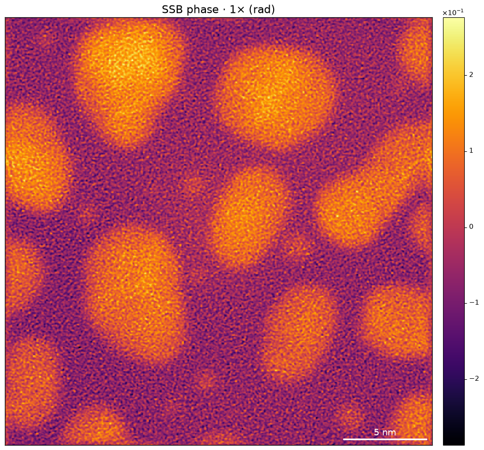
result.show() gives the phase its own large panel. result.show("probe") shows the real-space and Fourier-space model intensities side by side. All three views use linear contrast and calibrated scale bars.

The model uses the voltage, convergence semiangle, and fitted aberrations already stored in the result. It is not an independently retrieved probe. Fourier intensity shows the aperture; aberrations are encoded in its complex phase. Each probe panel uses its own full intensity range.

Use result.probe() or result.probe(space="fourier") to access the complex arrays directly.

result.show()

result.show("probe")

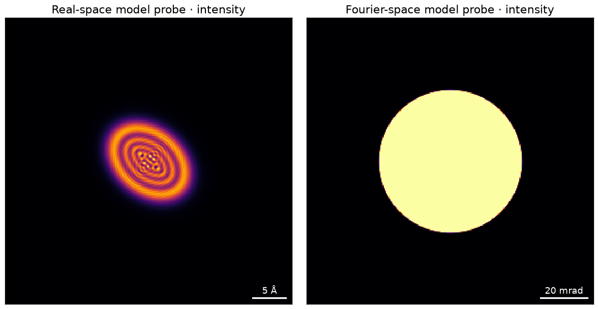
The two panels have different fields of view and independent contrast scales. The probe peaks at one; its colorbar is relative intensity. The object colorbar is phase in radians. The phase comes from experimental measurements, not known specimen potential; this example does not establish quantitative phase accuracy inside the thicker Gold particles.

Compare native and 4× phase sampling

The same fitted aberrations are applied at both output sampling factors. The library marks a central region on each full image and shows the matching crops underneath. All four panels share the native image’s full phase range. Change axsize to set the width and height of each panel in inches.

The finer output can expose bands and grid artifacts. More pixels do not establish improved physical resolution.

result_4x = ssb.reconstruct(aberrations, upsample=4, save_to="results/gold-ssb-4x")
result.show(compare=result_4x, axsize=(6, 6))

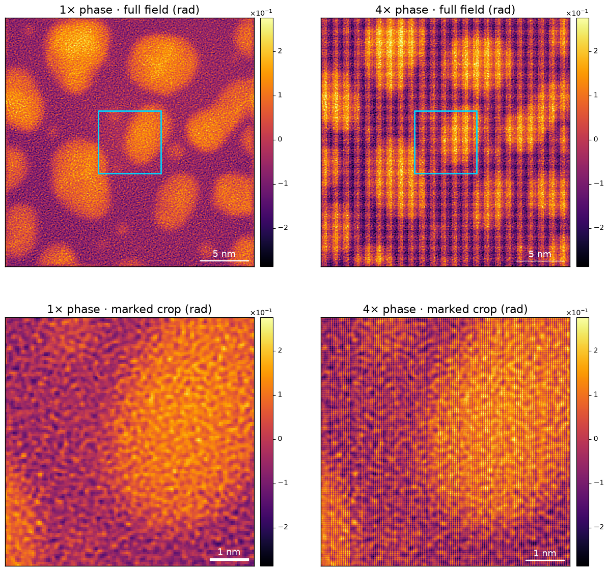
The 4× Gold result has vertical bands and does not demonstrate improved resolution. The earlier 2× test showed the same issue. Use 1× for this acquisition pending a validated implementation fix. The search parameters and model probe are unchanged; the additional output samples do not validate the new texture.

A separate diagnostic on 3 October 2026 traced the dominant stripes to replication of the mean-background Fourier term during upsampling: identical mean diffraction patterns at every scan position produced a flat 1× image but a striped 4× image. Removing that term before expansion suppressed the dominant stripes while leaving native phase unchanged within 3 × 10⁻⁸ rad. That was a diagnostic, not a released or fully validated correction; the saved plots here still show the original implementation.

Check ssb.scan_shape when changing inputs. The dense CUDA path may pad or crop unsupported scan grids; this 512 × 512 scan is unchanged. SSB grid limits distinguish that preparation from output upsampling.

Keep ssb open to inspect other reconstructions or search trials. Close it before the acquisition when finished. The QEM file and SSB results remain in results/.

ssb.close()
saved.close()