Mechanical behavior of structural materials (MSAE 4215) course notes (Draft)

Motivation

The following notes are derived from the MSAE 4215 course at Columbia University in Spring 2024 instructed by Dr. William Bailey. Equations and content were acquired from the instructor’s note packet and slides. The primary goal of this page is to enhance understanding before the midterm and use it a future reference for my research.

Lecture 2. Stress and torque tensor

Stress tensor

\[\begin{equation} [\sigma] = \begin{bmatrix} \sigma_{11} & \sigma_{12} & \sigma_{13} \\ \sigma_{21} & \sigma_{22} & \sigma_{23} \\ \sigma_{31} & \sigma_{32} & \sigma_{33} \\ \end{bmatrix} \end{equation}\]

Stress elements are assumed to be in equilibrium that there must be an equal and opposite stress acting on the parallel face. For a 3D problem, it should be then 9 instead of 18 due to symmetry. If there is no body force, we can further reduce down to 6 unique elements. In $\sigma_{ij}$, $i$ refers to the direction and $j$ refers to the plane.

Torque for homogenous stresses

Assume you have a cubic volume element of $\delta x^3$. The total torque is found using the below

\[\sum_i \textbf{r}_i \times \textbf{F}_i = \tau\]

where $\textbf{r}_i$ is the distance from center of the cubic volume element. Using the right hand rule, the net torque applied on a 2D plane is the following.

\[F = \sigma (\delta x^2)\] \[\tau = \textbf{r}_1 \times \textbf{F}_1 + \textbf{r}_2 \times \textbf{F}_2 + ... + \textbf{r}_i \times \textbf{F}_i\]

In a 2D plane stress situation, there are four shear stress components to consider. It is important to note that the distance from the origin to the point of interest is $\delta x/2$. Additionally, pay careful attention to the signs of the shear stresses, as the resulting torque is determined using the cross product.

\[\frac{\delta x}{2}(2 \sigma_{32} - 2\sigma_{23}) \delta x^2 = 0\]

Now, if there is no other force applied on the cubic element,

\[\sigma_{23} = \sigma_{32}\]

This can be generalized to

\[\sigma_{ij} = \sigma_{ji}\]

Torque for inhomoegenous stresses

Let us consider a system where body torques such as gravitational forces and stresses are inhomogenous.

Now each stress is a function of both $x_i$ and the slight Therefore the torque is the following.

\[\begin{equation} \begin{aligned} \tau_1 = & \frac{\delta x}{2}\bigg[\sigma_{32}\left(x_2 + \frac{\delta x}{2}\right) + \sigma_{32}\left(x_2 - \frac{\delta x}{2}\right) \\ & - \sigma_{23}\left(x_2 + \frac{\delta x}{2}\right) - \sigma_{23}\left(x_2 - \frac{\delta x}{2}\right) + G_1\bigg]\delta x^2 + G_{1} \delta x^3 \end{aligned} \end{equation}\]

Again, we are still looking at a cubic system. $\tau$ is the resulting net torque applied in the “1” direction.

Taylor-expand

Recall

\[y(x + ∆x) \approx y(x) + y'(x) ∆x\] \[\begin{align*} \sigma_{32}\left(x_2 + \frac{\delta x}{2}\right) + \sigma_{32}\left(x_2 - \frac{\delta x}{2}\right) &= 2 \sigma_{32}(x_2) + \frac{\partial \sigma_{32}}{\partial x_2} \frac{\delta x}{2} - \frac{\partial \sigma_{32}}{\partial x_2} \frac{\delta x}{2} \\ &= 2 \sigma_{32}(x_2) \end{align*}\] \[\begin{align} \tau_1 = (\sigma_{32} - \sigma_{23} + G_1) \delta x^3 \end{align}\]

If the net torque is zero in the choosen direction, then

\[\begin{align*} \sigma_{32} - \sigma_{23} + G_1 = 0 \end{align*}\]

Stress general expression

\[\begin{align} F_3 &= \left[\sigma_{33}\left(x_3 + \frac{\delta x}{2}\right) - \sigma_{33}\left(x_3 - \frac{\delta x}{2}\right) \right. \\ &\quad + \sigma_{32}\left(x_2 + \frac{\delta x}{2}\right) - \sigma_{32}\left(x_2 - \frac{\delta x}{2}\right) \\ &\quad + \left. \sigma_{31}\left(x_3 + \frac{\delta x}{2}\right) - \sigma_{31}\left(x_3 - \frac{\delta x}{2}\right)\right]\delta x^2 \\ &\quad + g_1\rho\delta x^3 \end{align}\]

Taylor expanding each of the $\sigma_{3i}$, and expressing $\delta x^3 = dV$

\[\frac{F_3}{dV} = \frac{\partial \sigma_{31}}{\partial x_1} + \frac{\partial \sigma_{32}}{\partial x_2} + \frac{\partial \sigma_{33}}{\partial x_3} + g_3\rho \tag{13}\]

Lecture 3. Principal axes of the stress tensor

Tensor definition

A 1-rank tensor is a 1D matrix, also known as a vector. A 2-rank tensor is a 2D matrix. A 3-rank tensor is a 3D matrix, and so on. Primarily, a tensor is used to transform vectors while maintaining a linear relationship between the two vectors.

\[\begin{align} \vec{p} = [T] \vec{q} \end{align}\]

Now, the following example is the relationship between the applied electric field $\vec{E}$ and currenty density $\vec{J}$. Here $\sigma$ is not stress but electrical conductivitiy.

\[\begin{equation} \begin{bmatrix} J_1 \\ J_2 \\ J_3 \end{bmatrix} = \begin{bmatrix} \sigma_{11} & \sigma_{21} & \sigma_{31} \\ \sigma_{21} & \sigma_{22} & \sigma_{32} \\ \sigma_{31} & \sigma_{32} & \sigma_{33} \end{bmatrix} \begin{bmatrix} E_1 \\ E_2 \\ E_3 \end{bmatrix} \end{equation}\]

In dummy suffix notation,

\[\begin{align} J_i = \sigma_{ij} E_i \end{align}\]

Now, to calculate the current density in a particular direction,

\[\begin{align} J_1 = \sigma_{11} E_1 + \sigma_{12} E_2 + \sigma_{13} E_3 \end{align}\]

Coordinate transformation via rotation

Rotate about single axis

On a 2D plane, assume a vector $\hat{x}_1$ points downwards and $\hat{x}_2$ points to the right, perpendicular to $\hat{x}_1$. Now, we want to rotate $\hat{x}_1$ and $\hat{x}_2$ about the normal to the plane axis $\hat{x}_3$ at a fixed angle. We want to know the resulting vectors transformed by the rotation.

\[\begin{equation} \begin{bmatrix} \hat{x}'_1 \\ \hat{x}'_2 \\ \hat{x}'_3 \end{bmatrix} = \begin{bmatrix} \cos \theta_3 & \sin \theta_3 & 0 \\ -\sin \theta_3 & \cos \theta_3 & 0 \\ 0 & 0 & 1 \end{bmatrix} \begin{bmatrix} \hat{x}_1 \\ \hat{x}_2 \\ \hat{x}_3 \end{bmatrix} \end{equation}\]

Recall we may set up the basis vector as

\[\hat{x}_1 = \begin{bmatrix} 1 \\ 0 \\ 0 \end{bmatrix}, \space \hat{x}_2 = \begin{bmatrix} 0 \\ 1 \\ 0 \end{bmatrix}, \space \hat{x}_3 = \begin{bmatrix} 0 \\ 0 \\ 1 \end{bmatrix}\]

Rotate about arbitrary axis

If we want to find the vectors transformed by rotation about arbitrary axes x, y, and z,

\[\begin{equation} \begin{bmatrix} \hat{x}'_1 \\ \hat{x}'_2 \\ \hat{x}'_3 \end{bmatrix} = R \begin{bmatrix} \hat{x}_1 \\ \hat{x}_2 \\ \hat{x}_3 \end{bmatrix} \end{equation}\]

where

\[\begin{equation} R = \begin{bmatrix} \cos \theta_3 & \sin \theta_3 & 0 \\ -\sin \theta_3 & \cos \theta_3 & 0 \\ 0 & 0 & 1 \end{bmatrix} \begin{bmatrix} \cos \theta_2 & 0 & \sin \theta_2 \\ 0 & 1 & 0 \\ -\sin \theta_2 & 0 & \cos \theta_2 \end{bmatrix} \begin{bmatrix} 1 & 0 & 0 \\ 0 & \cos \theta_1 & \sin \theta_1 \\ 0 & -\sin \theta_1 & \cos \theta_1 \end{bmatrix} \end{equation}\]

Cartesian to spherical coordinates

\[\begin{equation} \begin{bmatrix} p_r \\ p_\theta \\ p_\phi \end{bmatrix} = \begin{bmatrix} \sin \theta \cos \phi & \sin \theta \sin \phi & \cos \theta \\ \cos \theta \cos \phi & \cos \theta \sin \phi & -\sin \theta \\ -\sin \phi & \cos \phi & 0 \end{bmatrix} \begin{bmatrix} p_x \\ p_y \\ p_z \end{bmatrix} \end{equation}\]

Reverse transformation

\[\begin{align} \textbf{p}' = \textbf{A} \textbf{p} \end{align}\]

We want to find another matrix $\textbf{B}$ that transform $\textbf{p}’$ to $\textbf{p}$ with a matrix $\textbf{B}$.

Given the transformation

\[\begin{equation} \textbf{p}' = \textbf{A} \textbf{p} \end{equation}\]

we seek another matrix $\textbf{B}$ such that

\[\begin{equation} \textbf{p} = \textbf{B} \textbf{p}' \end{equation}\]

Substituting the first equation into the second gives

\[\begin{equation} \textbf{p} = \textbf{B} (\textbf{A} \textbf{p}) \end{equation}\]

For the identity transformation where $\textbf{p} = \textbf{I} \textbf{p}$, where $\textbf{I}$ is the identity matrix, it follows that

\[\begin{equation} \textbf{I} = \textbf{B} \textbf{A} \end{equation}\]

Therefore, matrix $\textbf{B}$ must be the inverse of matrix $\textbf{A}$, i.e., $\textbf{B} = \textbf{A}^{-1}$, provided that $\textbf{A}$ is an invertible matrix.

\[\begin{align} \textbf{p} = \textbf{B}\textbf{p}' \end{align}\]

Now we claim that due to the orthonormality conditions and inverse matrix,

\[\begin{align} b_{ij} = a_{ji} \end{align}\]

For the spherical to cartesian reverse transformation,

\[\begin{equation} \begin{bmatrix} p_x \\ p_y \\ p_z \end{bmatrix} = \begin{bmatrix} \sin \theta \cos \phi & \cos \theta \cos \phi & -\sin \phi \\ \sin \theta \sin \phi & \cos \theta \sin \phi & \cos \phi \\ \cos \theta & -\sin \theta & 0 \end{bmatrix} \begin{bmatrix} p_r \\ p_\theta \\ p_\phi \end{bmatrix} \end{equation}\]

Transformation beyond rank-1 tensor

We have so far studied transforming vectors using matrix elements. If we want to transform second-rank tensors or beyond, we may follow the procedure below. However, this topic is not fully expounded upon.

\[\begin{array}{|c|c|c|c|} \hline \text{Rank} & \text{Description} & \text{Forward} & \text{Reverse} \\ \hline 1 & \text{vector} & p'_i = a_{ij}p_j & p_i = a_{ji}p'_j \\ \hline 2 & \text{second-rank} & T'_{ij} = a_{ik}a_{jl}T_{kl} & T_{ij} = a_{ki}a_{lj}T'_{kl} \\ \hline 3 & \text{third-rank} & T'_{ijk} = a_{il}a_{jm}a_{kn}T_{lmn} & T_{ijk} = a_{li}a_{mj}a_{nk}T'_{lmn} \\ \hline \end{array}\]

Principal axes

In real space, we want to determine stress components applied to a system. There are 9 elements.

Here, it both includes shear stress and normal stress. But we want to remove shear stress and reorient the coordinate system to align with the principal axes. Here, the off-diagonal terms (shear stresses) become zero, and the only non-zero components are the normal stresses on the diagonal. These normal stresses are called the principal stresses.

Starting with the eigenvalue problem:

\[\begin{equation} \begin{bmatrix} \sigma_{11} & \sigma_{12} & \sigma_{13} \\ \sigma_{12} & \sigma_{22} & \sigma_{23} \\ \sigma_{13} & \sigma_{23} & \sigma_{33} \end{bmatrix} \begin{bmatrix} \hat{x}_1 \\ \hat{x}_2 \\ \hat{x}_3 \end{bmatrix} = \lambda \begin{bmatrix} \hat{x}_1 \\ \hat{x}_2 \\ \hat{x}_3 \end{bmatrix} \end{equation}\]

We find the eigenvalues and eigenvectors of the matrix. The eigenvectors form a matrix Q, and the eigenvalues form a diagonal matrix such that:

We may find the eigenvalues using the standard method below.

\[\begin{equation} \begin{vmatrix} \sigma_{11} - \lambda & \sigma_{12} & \sigma_{13} \\ \sigma_{12} & \sigma_{22} - \lambda & \sigma_{23} \\ \sigma_{13} & \sigma_{23} & \sigma_{33} - \lambda \end{vmatrix} = 0 \end{equation}\]

Where A is the original matrix and Q is the orthogonal matrix of eigenvectors.

The diagonalized matrix is:

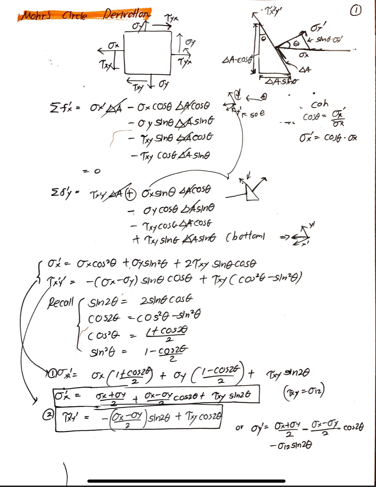
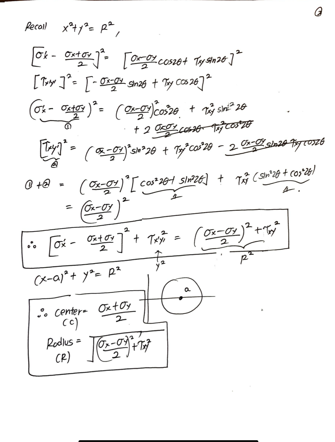
\[\begin{equation} \begin{bmatrix} \sigma_1 & 0 & 0 \\ 0 & \sigma_2 & 0 \\ 0 & 0 & \sigma_3 \end{bmatrix} \end{equation}\]

Morh’s circle derivations

I will type write later perhaps after the exam or after the semester.

Free body diagram Morh's circle derivation

Lecture 4. Strain tensor

In previous lectures, we discussed how to determine principle axises via coordinate transformation or solving an eigenvalue problem. Here, we will discuss how strain elements are affected due to stresss. Strain is the response to stress.

For uniform and unixial stress, we define tensile strain as

\[\begin{equation} \varepsilon = \frac{\Delta l}{l_o} \end{equation}\]

The above definition is general. We want to account for inhomogenous strains, shear strains, etc.

Imagine on a 1-D string, you have points $P$ and $Q$ with a separated by $\delta x$. If you stretch the string the two points will be shifted to $P’$ and $Q’$. Then, the new vector between $P’$ and $Q’$. The initial displacement between $P$ and $O$ is $u_1(x_1)$.

\[\begin{equation} \epsilon_1(x_1) = \frac{\overline{P'Q'} - \overline{PQ}}{\overline{PQ}} \end{equation}\]

$u(x_1)$ measures how much a point at $x_1$ has moved due to deformation.

$u(x_1 + \delta x)$ measures the displacement of another point that was originally a small differnece $\delta x$ away from $x_1$.

\[\begin{equation} \epsilon_1(x_1) = \frac{u_1(x_1 + \delta x_1) - u_1(x_1)}{\delta x_1} \end{equation}\] \[\begin{equation} \epsilon_1(u_1) = \frac{\partial u_1(x_1)}{\partial x_1} \end{equation}\]

For 2D strain

\[\begin{equation} \overline{PQ} = | \delta \textbf{x}| = \sqrt{(\delta x_1)^2 + (\delta x_2)^2} \end{equation}\] \[\begin{equation} \overline{P'Q'} = | \delta \textbf{x} + \delta \textbf{u} | = \sqrt{(\delta x_1 + \delta u_1)^2 + (\delta x_2 + \delta u_2)^2} \end{equation}\]

Use $\sqrt{a^2 + x} \approx a + x/2a$

\[\begin{equation} \overline{P'Q'} = | \delta \textbf{u} + \delta \textbf{x} | \approx | \delta \textbf{x}| + |\delta \textbf{x}|^{-1} (\delta u_1 \delta x_1 + \delta u_2 \delta x_2) \end{equation}\] \[\begin{equation} \overline{P'Q'} - \overline{PQ} \approx |\delta \textbf{x}|^{-1} (\delta u_1 \delta x_1 + \delta u_2 \delta x_2) \end{equation}\]

Evaluate $\delta u_1$ and $\delta u_2$ with full differentials.

\[\begin{align} \delta u_1 = \frac{\partial u_1}{\partial x_1} \delta x_1 + \frac{\partial u_1}{\partial x_2} \delta x_2 \\ \delta u_2 = \frac{\partial u_2}{\partial x_1} \delta x_1 + \frac{\partial u_2}{\partial x_2} \delta x_2 \end{align}\]

Let us introduce a strain term.

\[\begin{equation} e_{ij} = \frac{\partial u_i}{\partial x_j} \end{equation}\]

Therefore

\[\begin{align} \delta u_1 = e_{11} \delta x_1 + e_{12} \delta x_2 \\ \delta u_2 = e_{21} \delta x_1 + e_{22} \delta x_2 \end{align}\]

Now we may express $\epsilon_1$ as the following

\[\begin{align} \epsilon_1(x_1) &= \frac{\overline{P'Q'} - \overline{PQ}}{\overline{PQ}} \\ &= \frac{|\delta \textbf{x}|^{-1} (\delta u_1 \delta x_1 + \delta u_2 \delta x_2) }{\overline{PQ}} \\ &= | \delta \textbf{x}|^{-2} (\delta u_1 \delta x_1 + \delta u_2 \delta x_2) \\ &= | \delta \textbf{x}|^{-2} [e_{11} \delta x_1^2 + e_{12} \delta x_1 \delta x_2 + e_{21} \delta x_2^2 + e_{22} \delta x_1 \delta x_2] \\ &= | \delta \textbf{x}^{-2} | [ e_{11}(\delta x_2)^2 + e_{22} (\delta x_2)^2 + (e_{12} + e_{21}) \delta x_1 \delta x_2 ] \end{align}\]

But we want to remove the antisymmetric terms. Define a strain tensor $\varepsilon_{ij}$ as

\[\begin{align} \varepsilon_{12} = \varepsilon_{21} \equiv \frac{1}{2}(e_{12} + e_{21}) \\ \end{align}\]

For 2D,

\[\begin{equation} \begin{matrix} \end{matrix} \begin{bmatrix} \varepsilon \end{bmatrix} = \begin{bmatrix} \varepsilon_{11} & \varepsilon_{12} \\ \varepsilon_{21} & \varepsilon_{22} \\ \end{bmatrix} = \begin{bmatrix} e_{11} & \frac{1}{2}(e_{12} + e_{21}) \\ \frac{1}{2}(e_{12} + e_{21}) & e_{22} \\ \end{bmatrix} \end{equation}\]

For 3D,

\[\begin{equation} \begin{bmatrix} \varepsilon_{11} & \varepsilon_{12} & \varepsilon_{13} \\ \varepsilon_{21} & \varepsilon_{22} & \varepsilon_{23} \\ \varepsilon_{31} & \varepsilon_{32} & \varepsilon_{33} \\ \end{bmatrix} = \begin{bmatrix} e_{11} & \frac{1}{2}(e_{12} + e_{21}) & \frac{1}{2}(e_{13} + e_{31}) \\ \frac{1}{2}(e_{12} + e_{21}) & e_{22} & \frac{1}{2}(e_{23} + e_{32}) \\ \frac{1}{2}(e_{13} + e_{31}) & \frac{1}{2}(e_{23} + e_{32}) & e_{33} \\ \end{bmatrix} \end{equation}\]

Express in terms of engineering stress $\gamma_{ij}$.

\[\begin{equation} \begin{bmatrix} \varepsilon \end{bmatrix} = \begin{bmatrix} \epsilon_{x} & \gamma_{xy}/2 & \gamma_{xz}/2 \\ \gamma_{xy}/2 & \epsilon_{y} & \gamma_{yz}/2 \\ \gamma_{xz}/2 & \gamma_{yz}/2 & \epsilon_{z} \\ \end{bmatrix} \end{equation}\] \[\begin{equation} \gamma_{yz} = 2\varepsilon_{yz} \end{equation}\]

Here, antisymmetryic tensors $w_{ij}$

\[\begin{equation} w_{12} = - w_{21} \equiv \frac{1}{2}(e_{12} - e_{21}) \\ w_{ij} \equiv \frac{1}{2}(e_{ij} - e_{ji} ) \end{equation}\]

By insepction, notice that $e_{12} = \varepsilon_{12} + w_{12}$ and $e_{21} = \varepsilon_{12} - w_{12}$.

Dilation

Just like a 2D stress tensor, we may convert strain tensor into principal axes.

\[[\varepsilon] = \begin{bmatrix} \varepsilon_{11} & \varepsilon_{12} & \varepsilon_{13} \\ \varepsilon_{21} & \varepsilon_{22} & \varepsilon_{23} \\ \varepsilon_{31} & \varepsilon_{32} & \varepsilon_{33} \\ \end{bmatrix} \rightarrow \begin{bmatrix} \epsilon_{1} & 0 & 0 \\ 0 & \epsilon_{2} & 0 \\ 0 & 0 & \epsilon_{3} \\ \end{bmatrix}\]

Volume change can be found.

\[\begin{equation} \Delta \equiv \frac{\delta V}{V} = \frac{V' - V_0}{V_0} = \frac{(1 + \epsilon_1)(1 + \epsilon_2)(1 + \epsilon_3)L_1L_2L_3 - L_1L_2L_3}{L_1L_2L_3} \end{equation}\]

Dialation is invariant under matrix transformation.

\[\begin{equation} \Delta = \epsilon_1 + \epsilon_2 + \epsilon_3 \text{ (principal axes)} = \varepsilon_{11} + \varepsilon_{22} + \varepsilon_{33} \text{ (any axes)} \end{equation}\]

Lecture 5. Elasticity and thermodynamics

SKIP for now

Lecture 6. Anisotropic elasticity

We want to determine the strain based on the stress. We also need to form compliances $S_{ijkl}$, a 4th-rank tensor in 3D.

\[\begin{align} \varepsilon_{ij} &= \frac{1}{E} \sigma_{kl} \\ &= S_{ijkl} \sigma_{kl} \end{align}\]

We may use stiffnesses $C_{ijkl}$.

\[\begin{align} \sigma_{ij} &= E \varepsilon_{kl} \\ &= C_{ijkl} \varepsilon_{kl} \end{align}\]

Simple shear stress

Assume we apply $\sigma_{12}=\sigma_{21}=\tau_{xy}$.

\[\begin{align} \varepsilon_{12} &= S_{1211} \sigma_{11} + S_{1212} \sigma_{12} + S_{1221} \sigma_{21} + S_{1222} \sigma_{22} \\ &= S_{1212} \sigma_{12} + S_{1221} \sigma_{21} \\ &= (S_{1212} + S_{1221}) \tau_{xy} \end{align}\]

Although not proven at the momemnt, assume $S_{1212}=S_{1221}$ to be true.

Recall the definition of engineering strain.

\[\begin{align} \gamma_{xy} &= 2 \varepsilon_{12} \\ &= 4 S_{1212} \tau_{xy} \end{align}\]

Recall the definition of shear modulus $G$.

\[\begin{align} \tau_{xy} &= G \gamma_{xy} \\ G &= \frac{1}{4 S_{1212}} \end{align}\]

Finding invariant elements

There are a total of $3^4=81$ elements in $S_{ijkl}$ or $C_{ijkl}$. This number reduces down to 21 even before we apply the crtystal symmetry of the system.

Experimental inaccessibility

Recall

\[\begin{equation} \sigma_{ij} = C_{ijkl} \varepsilon_{kl} \end{equation}\]

Stress tensor elements are symmetric. We will not provide a proof at the moment.

\[\begin{equation} \therefore C_{ij\textbf{kl}} = C_{ij\textbf{lk}} \end{equation}\] \[\begin{equation} \therefore C_{\textbf{ij}kl} = C_{\textbf{ji}kl} \end{equation}\]

Instead of 9 times 9 unique elements, there will be 6 times 6 unqiue elements.

Thermodynamic restrictions

We now want to further reduce from 36 unique elements to 21 elements using thermodynamics.

For now, assume the following equation to be true.

\[\begin{equation} C_{\textbf{ij}kl} = C_{kl\textbf{ij}} \end{equation}\]

The above relationship indicates that

\[\begin{gather} \sigma_{ij} = C_{ijlk} \varepsilon_{kl} \\ \sigma_{kl} = C_{klij} \varepsilon_{ij} \\ \therefore \sigma_{11} = C_{1122} \varepsilon_{22} \\ \therefore \sigma_{22} = C_{2211} \varepsilon_{11} \\ \frac{\varepsilon_{11}}{\sigma_{22}} = \frac{\varepsilon_{22}}{\sigma_{11}} \end{gather}\]

Neumann’s principle

Rotate strains and stresses to new axes.
If the rotation is an element of the point group, the elastic tensor is the same. $[T]’ = [T]$.

To formally write:

\[T_{ijkl} = a_{im}a_{jn}a_{ko}a_{lp} T_{mnop}\]

Imagine we want to rotate $\theta= \pi/2$ about the z axis.

\[\begin{equation} a_{ij} = \begin{bmatrix} \cos \theta_3 & \sin \theta_3 & 0 \\ -\sin \theta_3 & \cos \theta_3 & 0 \\ 0 & 0 & 1 \end{bmatrix} = \begin{bmatrix} 0 & 1 & 0 \\ -1 & 0 & 0 \\ 0 & 0 & 1 \end{bmatrix} \end{equation}\] \[\begin{equation} a_{12} = 1 \quad a_{21} = -1 \quad a_{33} = 1 \end{equation}\]

Consider $S_{1111}$ for a cubic system with a 90-fold rotation symmetry.

\[S_{1111} = a_{1m} a_{1n} a_{1o} a_{1p} = S_{mnop}\]

Notice that the only $a_{12}=1$ is available. Therefore,

\[\begin{gather} S_{1111} = a_{12} a_{12} a_{12} a_{12} S_{2222} \\ \therefore S_{1111} = S_{2222} \\ \therefore S_{11} = S_{22} = S_{33} \end{gather}\]

Now, consider $S_{1122}$ and $S_{2211}$

\[\begin{gather} S_{1122} = a_{1m} a_{1n} a_{2o} a_{2p} S_{mnop} \\ \end{gather}\]

All elements are zero except $m=n=2$ and $o = p = 2$.

\[\begin{gather} S_{1122} = S_{2211} \\ \therefore S_{12} = S_{21} \end{gather}\]

Now consider $S_{2233}$.

\[S_{2233} = a_{2m} a_{2n} a_{3o} a_{3p} S_{mnop}\]

All elements are zero except $m = n = 1$ and $o = p = 3$.

Therefore,

\[\begin{gather} S_{2233} = S_{1133} \\ \therefore S_{23} = S_{13} \end{gather}\]

Consider $S_{63} \equiv S_{1233}$

\[\begin{equation} S_{1233} = a_{1m} a_{2n} a_{3o} a_{3p} S_{mnop} \end{equation}\]

Therefore, non-zero elements are when $m=2$, $n=1$, $o=p=2$.

\[\begin{gather} S_{1233} = 1 \times 1 \times -1 \times 1 = - S_{2133} \\ \therefore S_{1233} = - S_{2133} \end{gather}\]

Recall the symmetry relation.

\[\begin{equation} S_{ijkl} = S_{jikl} \end{equation}\] \[\begin{gather} S_{1233} = - S_{1233} \\ \therefore \boxed{S_{1233} = 0} \end{gather}\]