# Show1D — All Features Comprehensive demo of the interactive 1D viewer: spectra, profiles, convergence curves, multi-trace overlay, axis calibration, log scale, grid density, legend, peak detection with selectable peaks, mutation methods, and state persistence.

try:
    import google.colab
    !pip install -q -i https://test.pypi.org/simple/ --extra-index-url https://pypi.org/simple/ quantem-widget
except ImportError:
    pass  # Not in Colab, skip

try:
    %load_ext autoreload
    %autoreload 2
    %env ANYWIDGET_HMR=1
except Exception:
    pass  # autoreload unavailable (Colab Python 3.12+)

env: ANYWIDGET_HMR=1

import numpy as np, torch, json
from pathlib import Path
import quantem.widget
from quantem.widget import Show1D
device = torch.device("mps" if torch.backends.mps.is_available() else "cuda" if torch.cuda.is_available() else "cpu")
def make_eels_spectrum(n=512, seed=0):
    torch.manual_seed(seed)
    e = torch.linspace(-20, 800, n, device=device)
    zlp = 1000 * torch.exp(-0.5 * (e / 3) ** 2)
    plasmon = 200 * torch.exp(-0.5 * ((e - 15) / 5) ** 2) + 80 * torch.exp(-0.5 * ((e - 30) / 8) ** 2)
    bg = torch.where(e > 5, 5000 * (e.clamp(min=5) / 5) ** -2.5, torch.tensor(0.0, device=device))
    edge = torch.where(e > 532, 15 * ((e - 532).clamp(min=0) / 50) ** 0.4 * torch.exp(-(e - 532) / 200), torch.tensor(0.0, device=device))
    spec = (zlp + plasmon + bg + edge).cpu().numpy()
    return e.cpu().numpy().astype(np.float32), (spec + np.random.default_rng(seed).poisson(2, n)).astype(np.float32)
def make_edx_spectrum(n=1024, seed=0):
    torch.manual_seed(seed)
    e = torch.linspace(0, 20, n, device=device)
    spec = 500 * torch.exp(-0.3 * e) * (e + 0.1)
    for c, a, s in [(1.74, 800, 0.06), (4.51, 400, 0.08), (6.40, 600, 0.08), (8.04, 350, 0.09), (8.63, 200, 0.09)]:
        spec = spec + a * torch.exp(-0.5 * ((e - c) / s) ** 2)
    spec = spec.clamp(min=0).cpu().numpy()
    return e.cpu().numpy().astype(np.float32), (spec + np.random.default_rng(seed).poisson(3, n)).astype(np.float32)
def make_radial_profile(n=256, seed=0):
    torch.manual_seed(seed)
    q = torch.linspace(0, 15, n, device=device)
    profile = 50 * torch.exp(-0.5 * ((q - 3.5) / 1.5) ** 2)
    for c, a, s in [(2.0, 100, 0.15), (3.46, 60, 0.15), (4.0, 80, 0.15), (5.3, 40, 0.2), (6.93, 30, 0.2)]:
        profile = profile + a * torch.exp(-0.5 * ((q - c) / s) ** 2)
    profile = profile.cpu().numpy() + 5 * np.random.default_rng(seed).standard_normal(n)
    return q.cpu().numpy().astype(np.float32), np.maximum(profile, 0).astype(np.float32)
def make_convergence_curve(n=200, seed=0):
    torch.manual_seed(seed)
    epochs = torch.arange(n, dtype=torch.float32, device=device)
    loss = (10.0 * torch.exp(-0.02 * epochs) + 0.1).cpu().numpy()
    return epochs.cpu().numpy(), (loss + 0.05 * np.random.default_rng(seed).standard_normal(n)).astype(np.float32)
def make_beam_current(n=500, seed=0):
    torch.manual_seed(seed)
    t = torch.linspace(0, 60, n, device=device)
    current = 120 - 0.3 * t + 5 * torch.sin(0.1 * t)
    current = current + torch.where(t > 30, torch.tensor(8.0, device=device), torch.tensor(0.0, device=device))
    current = current.cpu().numpy() + 2 * np.random.default_rng(seed).standard_normal(n)
    return t.cpu().numpy().astype(np.float32), current.astype(np.float32)
print(f"Generators ready (device={device})")
print(f"quantem.widget {quantem.widget.__version__}")

Generators ready (device=mps)
quantem.widget 0.4.0a3

---

Single EELS Spectrum

Basic usage with calibrated energy axis and axis labels.

energy, spec = make_eels_spectrum()
Show1D(spec, x=energy, title="EELS — O-K Edge", x_label="Energy Loss", x_unit="eV", y_label="Counts")

EDX Spectrum

Energy-dispersive X-ray spectrum with characteristic peaks.

edx_energy, edx_spec = make_edx_spectrum()
Show1D(edx_spec, x=edx_energy, title="EDX Spectrum", x_label="Energy", x_unit="keV", y_label="Counts")

Radial Profile from Diffraction

Azimuthally averaged diffraction intensity vs. scattering vector.

q, profile = make_radial_profile()
Show1D(profile, x=q, title="Radial Profile", x_label="q", x_unit="1/nm", y_label="Intensity")

Multi-Trace Overlay — EELS Comparison

Compare spectra from different sample regions with distinct colors and legend.

specs = [make_eels_spectrum(seed=i)[1] for i in range(4)]
Show1D(
    specs,
    x=energy,
    labels=["Grain Interior", "Grain Boundary", "Precipitate", "Matrix"],
    title="EELS — Spatial Comparison",
    x_label="Energy Loss",
    x_unit="eV",
    y_label="Counts",
)

Log Scale — Convergence Curves

Compare different reconstruction algorithms on a log-scale Y axis.

epochs, loss1 = make_convergence_curve(seed=0)
_, loss2 = make_convergence_curve(seed=1)
_, loss3 = make_convergence_curve(seed=2)
loss2 = loss2 * 1.5
loss3 = loss3 * 0.7
Show1D(
    [loss1, loss2, loss3],
    x=epochs,
    labels=["ePIE", "rPIE", "ML-PIE"],
    title="Reconstruction Convergence",
    x_label="Iteration", y_label="Error", log_scale=True,
)

Auto-Contrast — Percentile Clipping

When the zero-loss peak dominates EELS spectra, core-loss edges are invisible. Auto-contrast clips the Y-axis to a configurable percentile range, revealing weak features without manual Y-range locking. Toggle the “Auto:” switch in the controls row, or set auto_contrast=True with custom percentile_low / percentile_high.

# Default view — ZLP dominates, core-loss edge invisible
energy, spec = make_eels_spectrum()
Show1D(spec, x=energy, title="EELS — Full Range (ZLP dominates)", x_label="Energy Loss", x_unit="eV", y_label="Counts")

# Auto-contrast — clips Y-axis to 2–98% percentile, revealing the O-K edge at 532 eV
Show1D(
    spec,
    x=energy,
    title="EELS — Auto-Contrast (2–98%)",
    x_label="Energy Loss",
    x_unit="eV",
    y_label="Counts",
    auto_contrast=True,
    percentile_low=2.0,
    percentile_high=98.0,
)

Custom Colors and Line Width

Show1D(
    [loss1, loss2],
    x=epochs,
    labels=["Adam", "SGD"],
    colors=["#e91e63", "#00bcd4"],
    title="Custom Colors",
    x_label="Epoch",
    y_label="Loss",
    line_width=2.5,
)

Beam Current Log

Monitor beam current drift over a TEM session.

t, current = make_beam_current()
Show1D(current, x=t, title="Beam Current", x_label="Time", x_unit="min", y_label="Current", y_unit="pA")

Hide Controls & Stats

Minimal view for publication or embedding.

Show1D(
    spec,
    x=energy,
    title="Clean View",
    x_label="Energy Loss",
    x_unit="eV",
    show_controls=False,
    show_stats=False,
    show_grid=False,
)

Simple Array (No X Axis)

When no X values are provided, indices are used.

t = torch.linspace(0, 4 * np.pi, 300, device=device)
Show1D(torch.sin(t).cpu().numpy().astype(np.float32), title="Sine Wave")

2D Array Input — Multiple Traces from Matrix

Pass a 2D array where each row is a trace.

x = torch.linspace(0, 2 * np.pi, 200, device=device)
phases = torch.linspace(0, np.pi, 5, device=device)
traces = torch.stack([torch.sin(x + p) for p in phases]).cpu().numpy().astype(np.float32)
Show1D(traces, x=x.cpu().numpy().astype(np.float32), title="Phase-Shifted Sinusoids", x_label="Angle", x_unit="rad")

---

Mutation — set_data()

Replace data while preserving display settings.

w = Show1D(spec, x=energy, title="Mutable Plot", x_label="Energy", log_scale=True)
w

# Replace with EDX data — log_scale and title are preserved
w.set_data(edx_spec, x=edx_energy)

Mutation — add_trace() / remove_trace()

w2 = Show1D(spec, x=energy, title="Add/Remove Demo")
w2

_, spec2 = make_eels_spectrum(seed=5)
_, spec3 = make_eels_spectrum(seed=10)
w2.add_trace(spec2, label="Region B")
w2.add_trace(spec3, label="Region C", color="#ff5722")

# Remove the first trace
w2.remove_trace(0)

---

State Persistence

Save and restore display settings across sessions.

w_save = Show1D(
    spec,
    x=energy,
    title="Saved State Demo",
    x_label="Energy Loss",
    x_unit="eV",
    log_scale=True,
    show_grid=False,
    line_width=2.0,
)
w_save.summary()

Saved State Demo
================================
Series:   1 x 512 points
Labels:   Data
X range:  -20 - 800
X axis:   Energy Loss (eV)
  [0] Data: mean=40.28  min=7.794e-06  max=3850  std=225.8
Display:  log

w_save.save("show1d_state.json")
print(json.dumps(w_save.state_dict(), indent=2))

{
  "title": "Saved State Demo",
  "labels": [
    "Data"
  ],
  "colors": [
    "#4fc3f7"
  ],
  "x_label": "Energy Loss",
  "y_label": "",
  "x_unit": "eV",
  "y_unit": "",
  "log_scale": true,
  "auto_contrast": false,
  "percentile_low": 2.0,
  "percentile_high": 98.0,
  "show_stats": true,
  "show_legend": true,
  "show_grid": false,
  "show_controls": true,
  "line_width": 2.0,
  "focused_trace": -1,
  "grid_density": 10,
  "x_range": [],
  "y_range": [],
  "peak_active": false,
  "peak_search_radius": 20,
  "peak_markers": [],
  "disabled_tools": [],
  "hidden_tools": []
}

# Restore from file — all display settings are preserved
w_loaded = Show1D(spec, x=energy, state="show1d_state.json")
w_loaded.summary()

Saved State Demo
================================
Series:   1 x 512 points
Labels:   Data
X range:  -20 - 800
X axis:   Energy Loss (eV)
  [0] Data: mean=40.28  min=7.794e-06  max=3850  std=225.8
Display:  log

# Cleanup
Path("show1d_state.json").unlink(missing_ok=True)

---

Peak Detection

Programmatically detect peaks using find_peaks(). Uses scipy.signal.find_peaks under the hood.

edx_energy, edx_spec = make_edx_spectrum()
w_peaks = Show1D(edx_spec, x=edx_energy, title="EDX — Peak Detection", x_label="Energy", x_unit="keV", y_label="Counts")
w_peaks.find_peaks(prominence=50)
print(f"Found {len(w_peaks.peaks)} peaks")
for pk in w_peaks.peaks:
    print(f"  {pk['x']:.2f} keV  (y={pk['y']:.0f})")
w_peaks

Found 5 peaks
  1.74 keV  (y=1348)
  4.52 keV  (y=996)
  6.39 keV  (y=1077)
  8.04 keV  (y=715)
  8.62 keV  (y=528)

Manual Peak Placement

Use add_peak() to place markers at specific X positions. The widget searches locally for the nearest maximum.

edx_energy, edx_spec = make_edx_spectrum()
w_manual = Show1D(edx_spec, x=edx_energy, title="Manual Peaks", x_label="Energy", x_unit="keV")
w_manual.add_peak(1.74, label="Si-K")
w_manual.add_peak(6.40, label="Fe-K")
w_manual.add_peak(8.04, label="Cu-K")
w_manual

Grid Density

Control the number of grid lines per axis. The grid slider (visible when grid is on) adjusts density from 5–50 lines.

# Show grid density control
energy, spec = make_eels_spectrum()
w_grid = Show1D(spec, x=energy, title="EELS — Dense Grid", x_label="Energy Loss", x_unit="eV", grid_density=25)
print(f"Grid density: {w_grid.grid_density} lines per axis")
w_grid

Grid density: 25 lines per axis

Selected Peaks

Click on peak markers to select them. Selected peak indices sync to Python via selected_peaks, and selected_peak_data returns the full marker dicts for downstream analysis.

edx_energy, edx_spec = make_edx_spectrum()
w_sel = Show1D(edx_spec, x=edx_energy, title="EDX — Selected Peaks", x_label="Energy", x_unit="keV")
w_sel.find_peaks(prominence=50)
w_sel.selected_peaks = [0, 1]
print(f"Selected indices: {w_sel.selected_peaks}")
print(f"Selected peak data:")
for pk in w_sel.selected_peak_data:
    print(f"  {pk['x']:.2f} keV  (y={pk['y']:.0f}, label={pk['label']})")
w_sel

Selected indices: [0, 1]
Selected peak data:
  1.74 keV  (y=1348, label=1.74)
  4.52 keV  (y=996, label=4.516)

Export Peaks

Export detected peaks to CSV or JSON for analysis in other tools.

edx_energy, edx_spec = make_edx_spectrum()
w_export = Show1D(edx_spec, x=edx_energy, title="Export Demo")
w_export.find_peaks(prominence=50)
csv_path = w_export.export_peaks("peaks.csv")
print(f"CSV exported to {csv_path}")
print(csv_path.read_text()[:300])
json_path = w_export.export_peaks("peaks.json")
print(f"\nJSON exported to {json_path}")
csv_path.unlink(missing_ok=True)
json_path.unlink(missing_ok=True)

CSV exported to peaks.csv
x,y,trace_idx,label,type
1.7399804592132568,1347.863525390625,0,1.74,peak
4.516129016876221,996.282958984375,0,4.516,peak
6.3929619789123535,1076.645263671875,0,6.393,peak
8.03519058227539,714.62939453125,0,8.035,peak
8.62170124053955,528.4463500976562,0,8.622,peak


JSON exported to peaks.json

Range-Scoped Statistics

Drag on the X axis to lock a range, or set x_range programmatically. When locked, the widget computes mean/min/max/std and integral within the selected region.

energy, spec = make_eels_spectrum()
w_range = Show1D(spec, x=energy, title="EELS — Range Stats", x_label="Energy Loss", x_unit="eV", y_label="Counts")
w_range.x_range = [500.0, 700.0]
print(f"Range stats: {w_range.range_stats}")
w_range

Range stats: [{'mean': 11.077767372131348, 'min': 0.04622071236371994, 'max': 17.93866729736328, 'std': 4.442169666290283, 'integral': 2193.355712890625, 'n_points': 124}]

Peak FWHM Measurement

Select peaks to measure their full width at half maximum via Gaussian fitting. Use measure_fwhm() for programmatic access.

edx_energy, edx_spec = make_edx_spectrum()
w_fwhm = Show1D(edx_spec, x=edx_energy, title="EDX — FWHM", x_label="Energy", x_unit="keV", y_label="Counts")
w_fwhm.find_peaks(prominence=50)
w_fwhm.measure_fwhm(peak_idx=0)
for f in w_fwhm.peak_fwhm:
    if f["fwhm"] is not None:
        print(f"Peak {f['peak_idx']}: FWHM = {f['fwhm']:.4f} keV, center = {f['center']:.3f} keV, R² = {f['fit_quality']:.4f}")
    else:
        print(f"Peak {f['peak_idx']}: fit failed — {f.get('error', 'unknown')}")
w_fwhm

Peak 0: FWHM = 0.1425 keV, center = 1.742 keV, R² = 0.9857

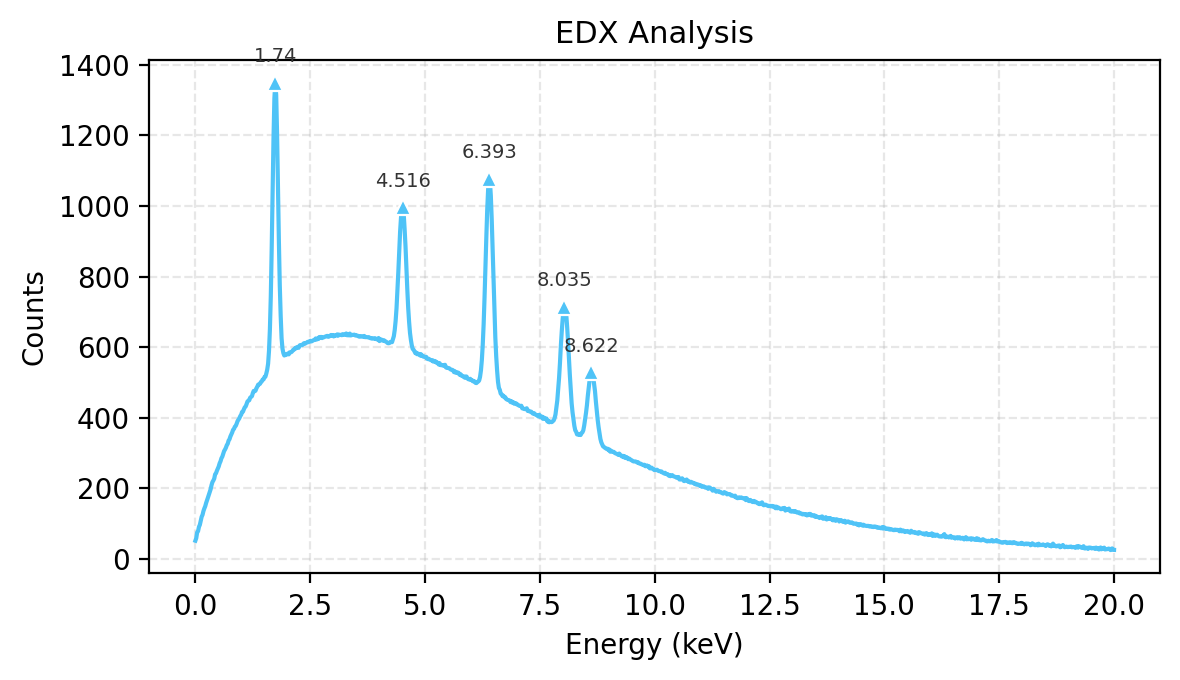
Publication Export — save_image()

Save publication-quality figures as PNG or PDF from Python. The JS Export dropdown also offers Figure (PDF) and Figure (PNG).

edx_energy, edx_spec = make_edx_spectrum()
w_fig = Show1D(edx_spec, x=edx_energy, title="EDX Analysis", x_label="Energy", x_unit="keV", y_label="Counts")
w_fig.find_peaks(prominence=50)
png_path = w_fig.save_image("edx_figure.png", dpi=200)
print(f"PNG: {png_path} ({png_path.stat().st_size / 1024:.0f} KB)")
pdf_path = w_fig.save_image("edx_figure.pdf", dpi=200)
print(f"PDF: {pdf_path} ({pdf_path.stat().st_size / 1024:.0f} KB)")
from IPython.display import Image, display
display(Image(filename=str(png_path), width=600))
png_path.unlink(missing_ok=True)
pdf_path.unlink(missing_ok=True)

PNG: edx_figure.png (71 KB)
PDF: edx_figure.pdf (22 KB)

---

Tool Lock / Hide

Disable or hide control groups programmatically. Useful for building guided workflows where only relevant controls are exposed.

# Hide export controls, disable peak tools
w_locked = Show1D(
    spec,
    x=energy,
    title="Locked Controls Demo",
    x_label="Energy Loss",
    x_unit="eV",
    hide_export=True,
    disable_peaks=True,
)
print(f"Hidden tools: {w_locked.hidden_tools}")
print(f"Disabled tools: {w_locked.disabled_tools}")
w_locked

Hidden tools: ['export']
Disabled tools: ['peaks']

# Apply a control preset — "spectroscopy" shows display + peaks + stats only
w_preset = Show1D(spec, x=energy, title="Spectroscopy Preset", x_label="Energy Loss", x_unit="eV")
w_preset.apply_control_preset("spectroscopy")
print(f"Hidden tools after preset: {w_preset.hidden_tools}")
w_preset

Hidden tools after preset: ['export']

---

Repr

w_repr = Show1D(
    [spec, edx_spec[:512]],
    x=energy,
    labels=["EELS", "EDX"],
    title="Final Demo",
    log_scale=True,
    line_width=1.5,
)
w_repr.find_peaks(prominence=50)
print(repr(w_repr))
w_repr.summary()

Show1D(2 traces x 512 points)
Final Demo
================================
Series:   2 x 512 points
Labels:   EELS, EDX
X range:  -20 - 800
  [0] EELS: mean=40.28  min=7.794e-06  max=3850  std=225.8
  [1] EDX: mean=507.8  min=52  max=1348  std=189.1
Display:  log | grid
Peaks:    2 markers