Getting Started#

Setup#

You need Python 3.11+, Node.js 20+, and the quantem core library.

Option A: conda (recommended)#

conda create -n widget python=3.12 nodejs=20 -y
conda activate widget
pip install quantem

git clone https://github.com/bobleesj/quantem.widget.git
cd quantem.widget
npm install
npm run build
pip install -e .

Option B: uv#

git clone https://github.com/bobleesj/quantem.widget.git
cd quantem.widget
npm install
npm run build
uv sync

Note: With uv, prefix Python commands with uv run, or activate with source .venv/bin/activate.

Verify#

python -c "from quantem.widget import Show2D; print('OK')"

Making changes#

JavaScript (layout, rendering, UI)#

npm run dev — watch mode, rebuilds on save
Set %env ANYWIDGET_HMR=1 in the notebook for live reload without re-running cells
Edit js/<widget>/index.tsx
Re-run the notebook cell (or let HMR pick it up automatically)

Python (data processing, observers)#

pip install -e . — once
Edit src/quantem/widget/<widget>.py
Restart the kernel and re-run cells.

Code organization#

Each widget is exactly one Python file + one TSX folder. No inheritance hierarchy — each widget is self-contained.

quantem.widget/
├── js/                          # TypeScript/React source
│   ├── align2d/index.tsx        # One folder per widget (each is self-contained)
│   ├── bin/index.tsx
│   ├── edit2d/index.tsx
│   ├── mark2d/index.tsx
│   ├── show1d/index.tsx
│   ├── show2d/index.tsx
│   ├── show3d/index.tsx
│   ├── show3dvolume/index.tsx
│   ├── show4d/index.tsx
│   ├── show4dstem/index.tsx
│   ├── showcomplex/index.tsx
│   ├── colormaps.ts             # ── Shared JS (used by all widgets) ──
│   ├── format.ts                #   Data extraction, number formatting
│   ├── histogram.ts             #   Histogram computation
│   ├── scalebar.ts              #   Scale bar, colorbar, figure export
│   ├── stats.ts                 #   Data statistics, log scale, clipping
│   ├── theme.ts                 #   Light/dark theme detection
│   ├── tool-parity.ts           #   Tool lock/hide logic
│   └── webgpu-fft.ts            #   GPU-accelerated FFT with CPU fallback
├── src/quantem/widget/          # Python source
│   ├── align2d.py               # One file per widget
│   ├── bin.py
│   ├── edit2d.py
│   ├── mark2d.py
│   ├── show1d.py
│   ├── show2d.py
│   ├── show3d.py
│   ├── show3dvolume.py
│   ├── show4d.py
│   ├── show4dstem.py
│   ├── showcomplex.py
│   ├── array_utils.py           # ── Shared Python (used by all widgets) ──
│   ├── json_state.py            #   State save/load envelope format
│   ├── tool_parity.py           #   Tool lock/hide validation
│   └── static/                  # Built JS bundles (generated by npm run build)
├── tests/                       # pytest unit tests + Playwright E2E tests
├── docs/                        # Sphinx documentation
├── notebooks/                   # Development/testing notebooks
├── package.json                 # esbuild config, npm scripts
└── pyproject.toml               # Python package config

Finding code is simple: Show4DSTEM’s Python is src/quantem/widget/show4dstem.py, its frontend is js/show4dstem/index.tsx.

Shared modules#

Each widget is self-contained, but a small set of utility modules are shared across all widgets. These exist because every widget needs them — they passed the bar of “used by 11+ widgets” before being extracted.

Python (src/quantem/widget/):

array_utils.py — to_numpy() converts any input (NumPy, PyTorch, CuPy) to NumPy. Used by all 11 widgets.
json_state.py — save_state_file() and unwrap_state_payload() for the versioned JSON state envelope. Used by all 11 widgets.
tool_parity.py — validates disabled_tools / hidden_tools keys. Used by 11 widgets.

JavaScript (js/):

theme.ts — useTheme() hook for automatic light/dark mode. Used by all 11 widgets.
colormaps.ts — colormap LUTs and applyColormap(). Used by all image widgets.
format.ts — extractFloat32(), formatNumber(), downloadBlob(). Used by all widgets.
stats.ts — computeStats(), percentileClip(), applyLogScale(). Used by all image widgets.
scalebar.ts — drawScaleBarHiDPI(), exportFigure(). Used by all canvas widgets with calibration.
histogram.ts — computeHistogramFromBytes(). Used by all image widgets.
webgpu-fft.ts — GPU-accelerated 2D FFT with CPU fallback. Used by all FFT-capable widgets.
tool-parity.ts — tool lock/hide state management. Used by 11 widgets.

Do not create new shared modules unless the logic is already duplicated across many widgets. When in doubt, keep it in the widget file and extract later.

Python ↔ JavaScript bridge#

anywidget bridges the two sides. You declare traitlets in Python, and they automatically sync to React state in the browser.

anywidget architecture: Python ↔ JavaScript bridge

Python declares traitlets#

Every trait marked .tag(sync=True) is visible to both Python and JavaScript:

class Show4DSTEM(anywidget.AnyWidget):
    pos_row = traitlets.Int(0).tag(sync=True)          # scalar → number
    frame_bytes = traitlets.Bytes(b"").tag(sync=True)   # binary → DataView

JavaScript reads and writes traitlets#

useModelState() works like useState but the value is synced to Python:

const [posRow, setPosRow] = useModelState<number>("pos_row");
const [frameBytes] = useModelState<DataView>("frame_bytes");  // read-only

Calling setPosRow(5) in JavaScript sets pos_row = 5 on the Python object.

Python reacts to changes#

.observe() registers callbacks that fire when a trait changes:

self.observe(self._update_frame, names=["pos_row", "pos_col"])

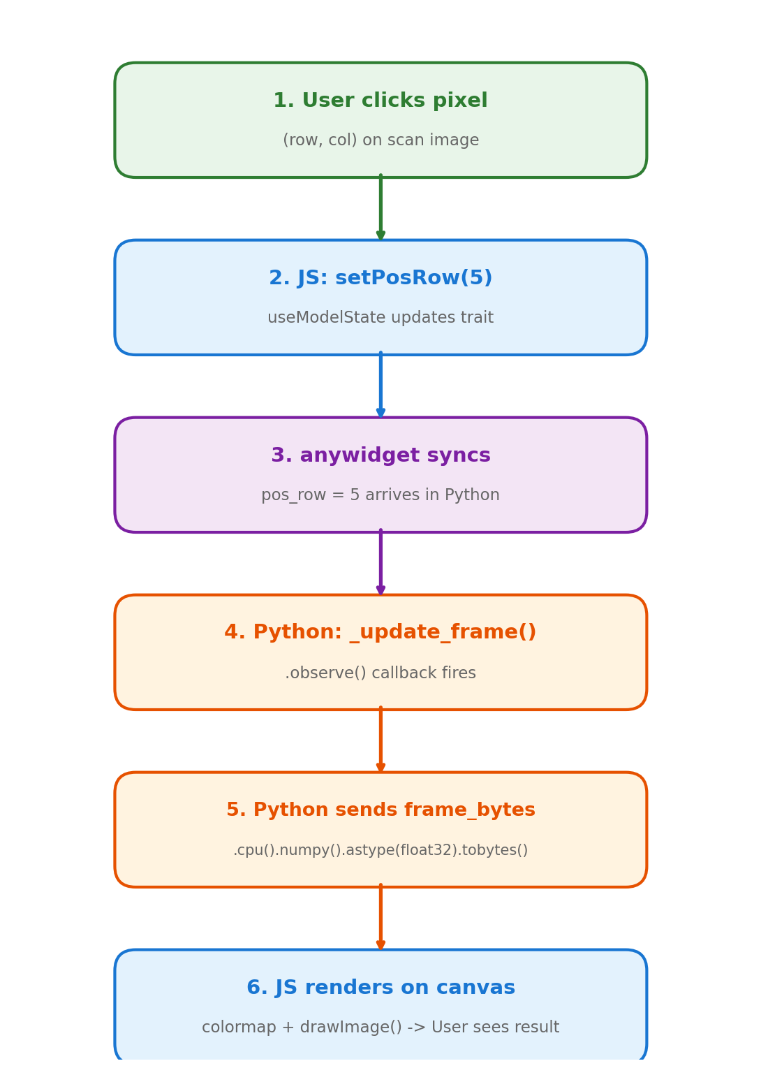
The full cycle#

When a user clicks a position on the scan image:

JS: user clicks → setPosRow(5) fires
Python: .observe() triggers _update_frame()
Python: extracts the frame, sets self.frame_bytes = ...
JS: receives new DataView, re-renders the canvas

This round-trip happens in milliseconds.

Trait types#

Python type	JS type	Example use
`traitlets.Int`	`number`	Position, shape, indices
`traitlets.Float`	`number`	Calibration, ROI params
`traitlets.Bool`	`boolean`	Toggles (log scale, ROI active)
`traitlets.Unicode`	`string`	Mode selection, titles
`traitlets.Bytes`	`DataView`	Image data (raw float32)
`traitlets.List`	`Array`	Compound updates, statistics

Data flow: GPU to browser#

The full dataset (potentially 16+ GB) stays on GPU or CPU as a PyTorch tensor. On each user interaction, Python extracts a single frame (~64 KB), serializes it as raw bytes, and sends it to the browser. The browser does colormapping and rendering entirely in JavaScript.

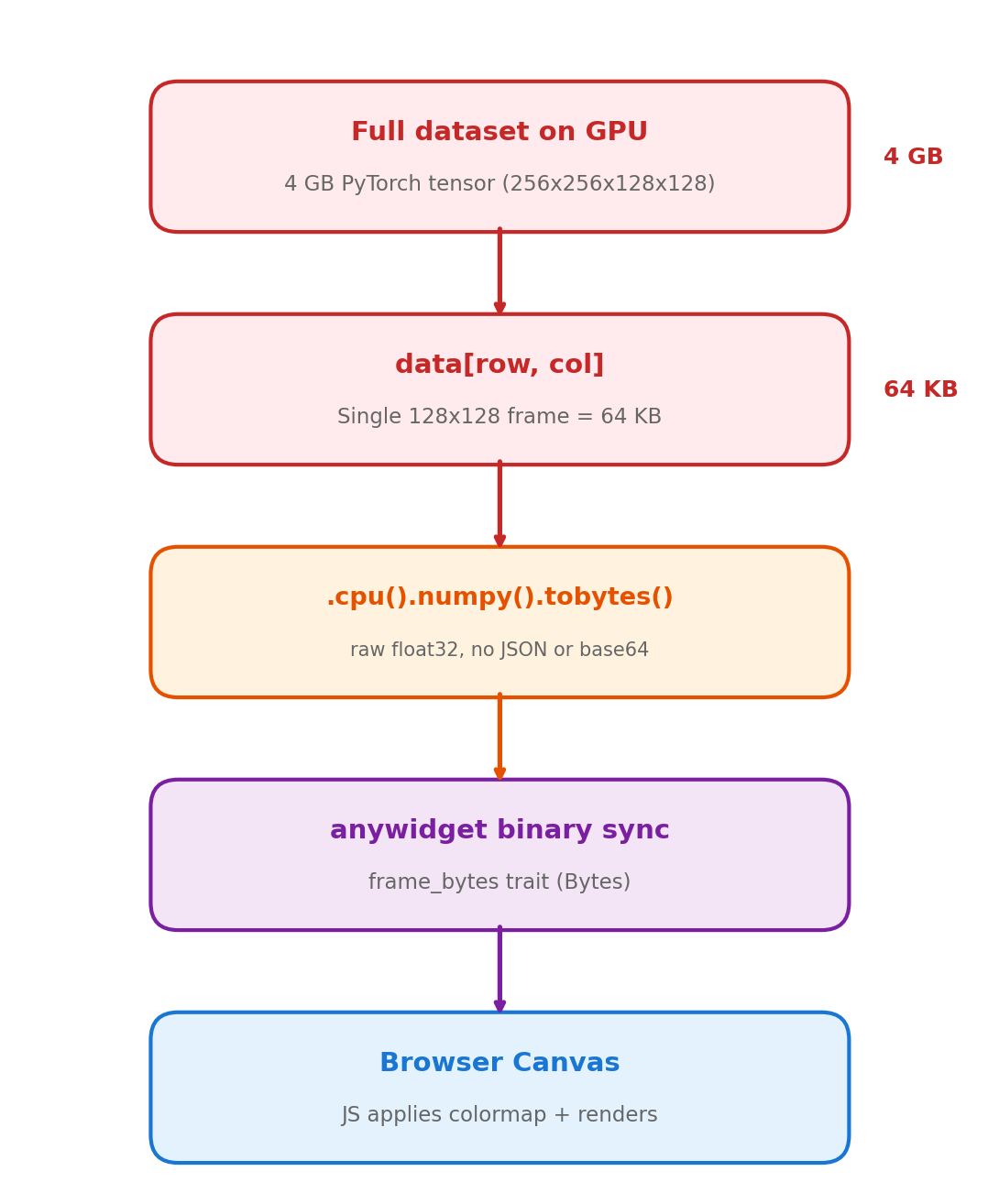
Data flow: full dataset on GPU, single frame to browser

A 16 GB dataset lives on GPU, but only 64 KB crosses the wire per click.

Widget catalog#

Widget	Description	GPU
`Show1D`	1D trace viewer with multi-trace overlay, crosshair, legend	No
`Show2D`	2D image viewer with gallery, ROI, line profiles, FFT, export	No
`Show3D`	3D stack viewer with playback, ROI, FFT, export	No
`Show3DVolume`	Orthogonal slice viewer (XY, XZ, YZ) with FFT, playback	No
`Show4D`	General 4D dataset explorer with nav + signal panels, ROI masking	Yes
`Show4DSTEM`	4D-STEM diffraction viewer with virtual imaging, ROI presets	Yes
`ShowComplex2D`	Complex-valued 2D viewer (amplitude/phase/HSV/real/imag)	No
`Mark2D`	Interactive 2D annotation (points, ROIs, profiles, snap-to-peak)	No
`Edit2D`	Interactive crop/pad/mask editor with brush tool	No
`Align2D`	Image alignment overlay with FFT-based auto-align	No
`Bin`	Detector binning with live preview and batch export	Yes