Fourier transform

It’s integeral transform that takes a function as input then ouputs another function that describes which frequenties are present in the original function

Definition

Allow you to transform any periodic function into a sum of sines and cosines.

Jean Baptiste Joseph Fourier (1768–1830)

\(F(u)\) holds the amplitude and phase of the sinusoid of frequency \(u\).

\[\begin{split}\begin{align} F(u) &= \int_{-\infty}^{\infty} f(x)\, e^{-i2\pi u x}\, dx, \\ F(u) &= \Re\{F(u)\} + i\,\Im\{F(u)\}. \end{align}\end{split}\]

The amplitude is

\[A(u) = \sqrt{ \Re\{F(u)\}^2 + \Im\{F(u)\}^2 }.\]

and the phase is

\[\phi(u) = \tan^{-1}\!\left(\frac{\Im\{F(u)\}}{\Re\{F(u)\}}\right).\]

Discrete Fourier Transform (DFT)

Recall the continuous Fourier transform in time:

\[X(F) = \int_{-\infty}^{\infty} x(t)\, e^{-i2\pi F t}\, dt.\]

The discrete version is

\[X_k = \sum_{n=0}^{N-1} x_n\, e^{-i2\pi \frac{k n}{N}},\]

where

\[\frac{k}{N} \approx F, \qquad n \approx t.\]

Here:

\(N\) is the total number of samples.
\(k\) is the frequency index, ranging from \(0\) to \(N-1\).
\(X_k\) is generally complex, representing both amplitude and phase of frequency component \(k\).

Expanding the sum using Euler’s formula \(e^{-i\theta} = \cos(\theta) - i\sin(\theta)\):

\[\begin{split}\begin{align} X_k &= \sum_{n=0}^{N-1} x_n \left[\cos\!\left(2\pi\frac{k n}{N}\right) - i \sin\!\left(2\pi\frac{k n}{N}\right)\right] \\ &= A_k + i B_k, \end{align}\end{split}\]

where \(A_k\) and \(B_k\) correspond to the real and imaginary parts, respectively.

At the end, you obtain a complex number \(X_k\), which can be plotted on the complex plane.

The magnitude \(|X_k|\) gives the amplitude, and the angle \(\arg(X_k)\) gives the phase.

Computing \(X_k\) in Practice

Imagine you have a simple \(\sin(x)\) function from \(0\) to \(2\pi\). You then sample, for example, 5 points — that is, \(N=5\).

Assume you want to compute \(X_1\) (so \(k=1\)). You know \(N\), and you have all values of \(x_n = \sin(x_n)\) for \(n=0,1,2,3,4\). You plug them into

\[X_k = \sum_{n=0}^{N-1} x_n\, e^{-i2\pi \frac{k n}{N}}.\]

At the end, you’ll get a complex number representing that frequency component.

You would then repeat the process for \(k=2,3,4,\) and so on.

How many \(k\) Values?

If you have \(N\) samples, then you can compute \(N\) discrete frequency components:

\[k = 0, 1, 2, \dots, N-1.\]

However:

Because the DFT of real-valued signals is symmetric, you typically only need to examine up to \(k = N/2\) (the “positive frequencies”).
The other half (\(k > N/2\)) contains the complex-conjugate mirror of those components.

So, for \(N = 5\), you can compute \(k = 0, 1, 2, 3, 4\), but often interpret only the first \(\lfloor N/2 \rfloor\) as unique frequency components.

How would you do this in 2D?

Let \(f(x,y)\) be a continuous function of spatial coordinates \(x, y\). Its 2D Fourier transform is

\[F(u,v) = \iint_{-\infty}^{\infty} f(x,y)\,e^{-i\,2\pi\,(u x + v y)}\,dx\,dy,\]

where \(u, v\) are the spatial frequencies (cycles per unit length) along \(x\) and \(y\).

The inverse transform is

\[f(x,y) = \iint_{-\infty}^{\infty} F(u,v)\,e^{+i\,2\pi\,(u x + v y)}\,du\,dv.\]

Discrete 2D DFT (samples on an \(M\times N\) grid)

Assume you have discrete samples \(f[x,y]\) for

\[x=0,1,\dots,M-1,\qquad y=0,1,\dots,N-1,\]

and you want their 2D DFT \(F[u,v]\) defined at the discrete frequency indices

\[u=0,1,\dots,M-1,\qquad v=0,1,\dots,N-1.\]

DFT:

\[F[u,v] = \sum_{x=0}^{M-1}\sum_{y=0}^{N-1} f[x,y]\;e^{-i\,2\pi\left(\frac{u x}{M}+\frac{v y}{N}\right)}.\]

Inverse DFT (IDFT):

\[f[x,y] = \frac{1}{MN}\sum_{u=0}^{M-1}\sum_{v=0}^{N-1} F[u,v]\;e^{+i\,2\pi\left(\frac{u x}{M}+\frac{v y}{N}\right)}.\]

Example with numpy

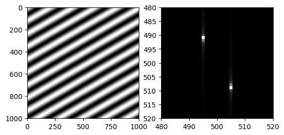
Here is an example of 2D Fourier transform where frequencies/pixels are shown as dots below:

[ ]:

# Source: https://thepythoncodingbook.com/2021/08/30/2d-fourier-transform-in-python-and-fourier-synthesis-of-images/
import numpy as np
import matplotlib.pyplot as plt

x = np.arange(-500, 501, 1)

X, Y = np.meshgrid(x, x)

wavelength = 100
angle = np.pi/3
grating = np.sin(
    2*np.pi*(X*np.cos(angle) + Y*np.sin(angle)) / wavelength
)

plt.set_cmap("gray")

plt.subplot(121)
plt.imshow(grating)

# Calculate Fourier transform of grating
# Shift the zero-frequency component to the center
ft = np.fft.fft2(grating)
ft = np.fft.fftshift(ft)

plt.subplot(122)
plt.imshow(abs(ft))
plt.xlim([480, 520])
plt.ylim([520, 480])  # Note, order is reversed for y
plt.show()