Statistics over many CIFs

Statistics over many CIFs#

A single .cif gives you geometry for one structure (physical features). When you have a folder, CifEnsemble is the hands-on tool: clean the set, see what is in it, filter, plot histograms, and copy matching files into new folders.

Elemental composition features are not from these CIFs - use OLED (Data in Brief table).

What data is on this page?#

Content	Source
Runnable demo (2 files)	Packaged GdSb + HoSb (`Example.demo_cif_folder_path`) - always available offline
Large structure / CN histograms	Figures from published / JOSS-scale ensembles - illustrative, not re-run here

If you no longer have a large private CIF collection on disk, you can still learn the API on the two-file demo and see what large runs look like from the figures. The same calls scale: tens of thousands of CIFs in SAF/CAF workflows, with cifkit as the geometry engine (Digital Discovery).

1. Work on a copy (hands-on setup)#

Preprocessing can rewrite ill-formatted files in place, and move_cif_files relocates them. Always work on a scratch copy:

import os
import shutil

from cifkit import CifEnsemble, Example

scratch = "demo_cifs"
os.makedirs(scratch, exist_ok=True)
for name in os.listdir(Example.demo_cif_folder_path):
    if name.endswith(".cif"):
        shutil.copy(os.path.join(Example.demo_cif_folder_path, name), scratch)

ensemble = CifEnsemble(scratch)

What just happened: cifkit walked the folder, preprocessed each CIF for gemmi compatibility, reported how many landed in error_* folders, then built a Cif object per file.

CIF Preprocessing in demo_cifs begun...

Preprocessing demo_cifs/GdSb.cif (1/2)
Preprocessing demo_cifs/HoSb.cif (2/2)

SUMMARY
# of files moved to 'error_*' folders: 0 (all clean)

Initializing 2 Cif objects...
Finished initialization!

With two clean rocksalt pnictides, you are ready to ask questions of the set - not of one file at a time.

2. “What is in this folder?”#

import pandas as pd

print("file_count:", ensemble.file_count)
print("unique_formulas:", ensemble.unique_formulas)
print("unique_structures:", ensemble.unique_structures)
print("unique_space_group_names:", ensemble.unique_space_group_names)
print("unique_elements:", ensemble.unique_elements)

Turn the same facts into a small table you can paste into a notebook or report:

overview = pd.DataFrame(
    [
        ("file_count", ensemble.file_count),
        ("unique_formulas", sorted(ensemble.unique_formulas)),
        ("unique_structures", sorted(ensemble.unique_structures)),
        ("unique_space_group_names", sorted(ensemble.unique_space_group_names)),
        ("unique_elements", sorted(ensemble.unique_elements)),
    ],
    columns=["stat", "value"],
)
print(overview.to_string(index=False))

stat	value
file_count	2
unique_formulas	[‘GdSb’, ‘HoSb’]
unique_structures	[‘NaCl’]
unique_space_group_names	[‘Fm-3m’]
unique_elements	[‘Gd’, ‘Ho’, ‘Sb’]

Reading the result (demo story): two formulas, one structure type (NaCl), one space group, three elements. On a real database dump you would see dozens of structure types and space groups here - same API, bigger folder.

Per-file series also exist (formula_stats, minimum_distances, supercell_atom_counts, …) - see the CifEnsemble API.

3. “Give me only the files that match …”#

Filters return paths (sets), so you can chain logic or hand them to copy/move:

print(ensemble.filter_by_formulas(["GdSb"]))
print(ensemble.filter_by_elements(["Ho"]))
print(ensemble.filter_by_space_group_names(["Fm-3m"]))

{'demo_cifs/GdSb.cif'}
{'demo_cifs/HoSb.cif'}
{'demo_cifs/GdSb.cif', 'demo_cifs/HoSb.cif'}

Hands-on read: GdSb-only is one path; Ho-containing is the other; space group Fm-3m is both. Other filters include structure, space-group number, composition type, site-mixing type, CN ranges, min distance, and supercell size.

4. “Park the matches in a new folder”#

ensemble.copy_cif_files(ensemble.filter_by_formulas(["GdSb"]), "sorted_GdSb")
print(os.listdir("sorted_GdSb"))

['GdSb.cif']

This is the usual lab pattern: filter a large dump, copy the hits into sorted_* for the next notebook or for SAF/CAF featurization.

5. “Show me the distribution” (histograms)#

On the demo (2 files) a structure histogram is almost trivial - both are NaCl - but the call is what you reuse on large sets:

ensemble.generate_structure_histogram(output_dir="histograms")
print(os.listdir("histograms"))

['structures.png']

Available histograms: structure, formula, tag, space group number and name, supercell size, elements, CN by both method families, composition type, and site mixing type.

What a larger ensemble looks like#

These figures are not recomputed from the two-file demo. They show the kind of output you get when the folder is big enough for histograms to matter.

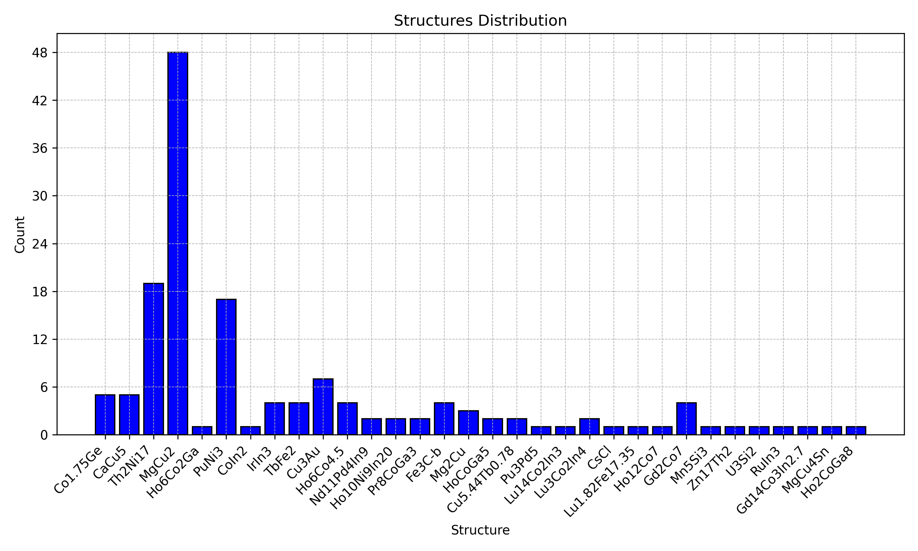
Structures distribution histogram from CifEnsemble — Fig. 4 **Structure histogram** from a larger ensemble via `generate_structure_histogram`. Same method as above; different folder size.#

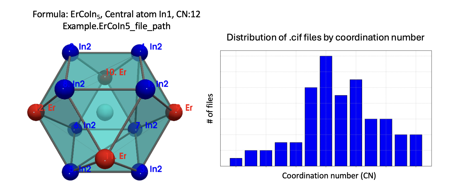
JOSS Figure 1 polyhedron and CN histogram — Fig. 5 **JOSS Figure 1.** One CIF polyhedron (left) and ensemble CN distribution (right) - the single-file vs many-file story on one page.#

Scale (when you do have thousands of files)#

Scale	What to expect
Demo (2 CIFs)	Seconds - this tutorial
~10,000 CIFs	Roughly 30-60 minutes on a laptop (supercell + neighbors per file)
SAF + CAF training tables	Tens of thousands of CIFs; feature tables on the order of a million rows (Digital Discovery); `cifkit` supplies the geometry

You do not need the large dataset to learn the API. You need it only when you want to regenerate large histograms or feature matrices yourself.

API#

Full method list: CifEnsemble.

Next#

Parse physical features from a .cif - distances, CN, polyhedra
OLED - elemental / composition features (dataset table, not from CIF)

Notes (demo data, citation)#

Runnable numbers on this page use packaged GdSb and HoSb only.
Large histograms are published / JOSS figures for orientation.
Soft cite for geometry / ensemble work: cifkit (JOSS); for feature-generation workflows also SAF + CAF (Digital Discovery). CITATION.txt · home page.